In this previous post, I wrote about the language of causal inference via counterfactuals. I briefly mentioned that there are at least two ways to capture the causal effect: counterfactuals and structural causal model. In this post, we are going to look at structural causal model and how we can use it to simulate what would happen if we do an intervention to a particular variable of interest. Please do note that both counterfactuals and structural causal model are highly overlapped and they share the same underlying concepts.

Simpson’s paradox in an acyclic directed graph

I have mentioned about simpson’s paradox briefly in my previous blog post. Here I am going to illustrate another perspective on how simpson’s paradox can affect the result of classical machine learning. Consider a (true) causal graph below.

Assume that we have data with these 5 variables in a spreadsheet style (think pandas dataframe) and we are tasked to find the effect on how exposure to sun (\(T\)) on the illness (\(Y\)). Without any knowledge of causal inference, we might think to just incorporate \(T\) as feature and create a linear regression model on the label \(Y\). Once we have the model, we use the coefficient to gauge and measure the relationship between exposure to sun and illness. If the coefficient is a positive number, then it tells us that there is a positive relationship, and vice versa if the coefficient is a negative number.

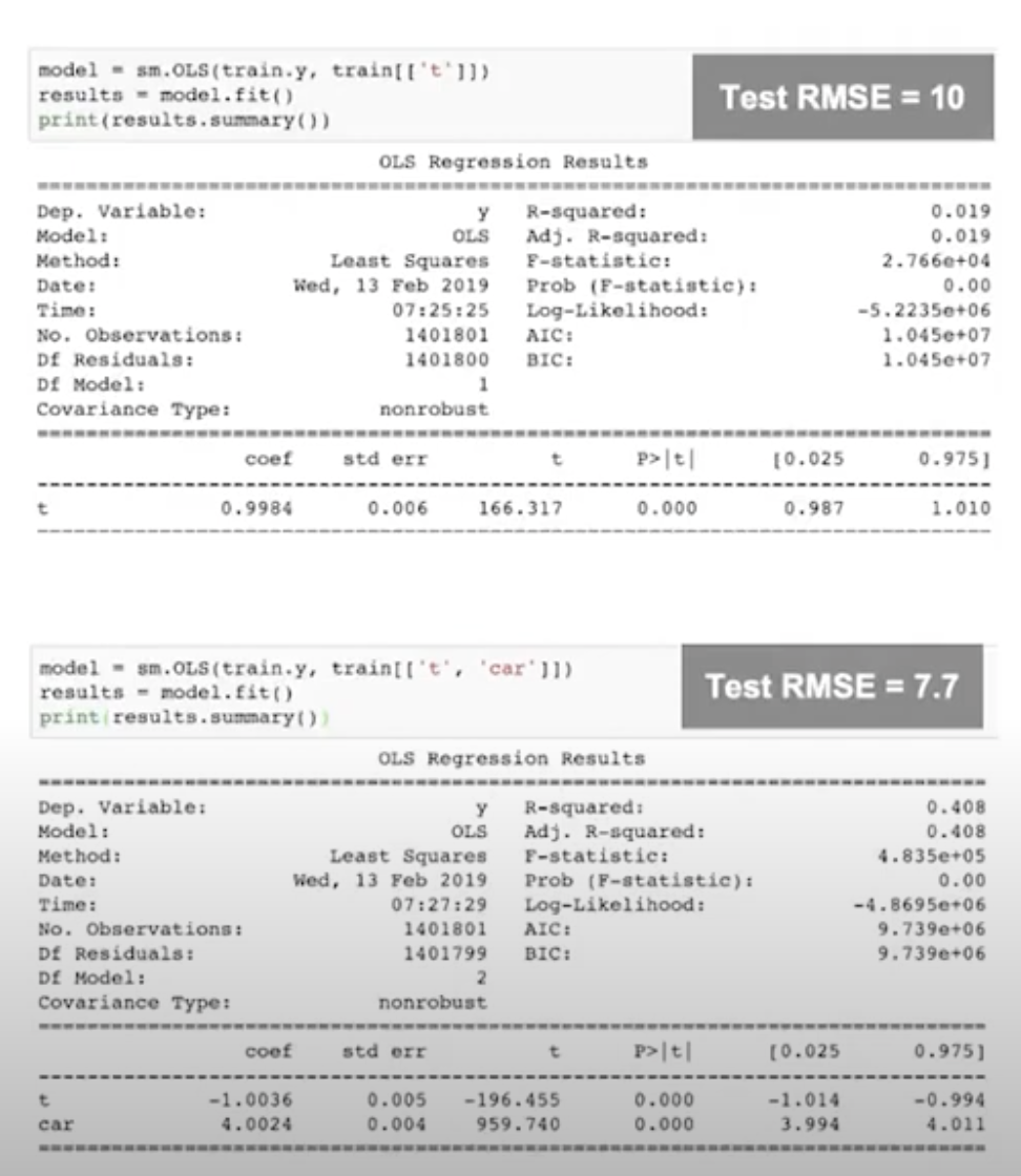
Looking at Figure 2 above, if we use \(T\) as the single feature to predict \(Y\), we got test RMSE of 10 and a coefficient of 0.99, meaning that there is a positive relationship between exposure to sun and illness. But if we were to add \(C\) (type of car owned) as feature, then we would have an even better test RMSE of 7.7, hinting that type of car owned is helpful in predictive power. But if we inspect the coefficient, we see that now \(T\) and \(Y\) have a negative relationship, whereas \(C\) and \(Y\) have a positive relationship. How can this happen? How can knowing the type of car owned results in more predictive power to illness? To the naked eye, this seems pretty unintuitive. But if we know the true causal graph we will immediately realized that knowing \(C\) indirectly tells us the age of the person, which gives it the predictive power to illness. This is another example of simpson’s paradox in a acyclic directed graph which we can use to distinguish flow of correlation vs causation.

Bayesian Network

We know that strong correlation between variables do not imply a causal effect. With counterfactuals, we introduce potential outcomes \((Y1, Y0)\) to be able to capture the causal effect. With structural causal model (SCM), the goal is to model the causal interdependencies between variables. One tool that we can use to achieve this is to use probabilistic graphical models (PGM). With PGM, we can model the relationships between features. PGM as a term encompasses many different approaches. In our case, one of the graph models that we can use to capture causal model is a bayesian network. Bayesian network is a directed acyclic graph that captures the interdependencies between variables. Nodes represent random variables, whereas edges represent relationships (the conditional probabilities) between variables.

In a bayesian network, the value of a node is independent of the rest of the variables in the graph given its parents. The relationship between arbitrary nodes are not necessarily causal. Therefore, we need to assume that the directed edges are the actual causal effect. This is where the unconfoundedness assumption plays in SCM. We need to believe and be sure that the bayesian network that we build have no unmeasured confounders.

How to build bayesian network?

So now we might ask: how do we build this bayesian network? If we have a lot of features, do we need to manually specify the causal relationships between the features that we have? There are some ways in which we can utilize correlation to automatically build the bayesian network, such as the NOTEARS algorithm. This automatic training is also known as structure learning. However, we can’t just blindly use the result. It’s better to have an expert to review the structure and fix the relationship (add, remove, or flip edges) in the bayesian network if deemed necessary.

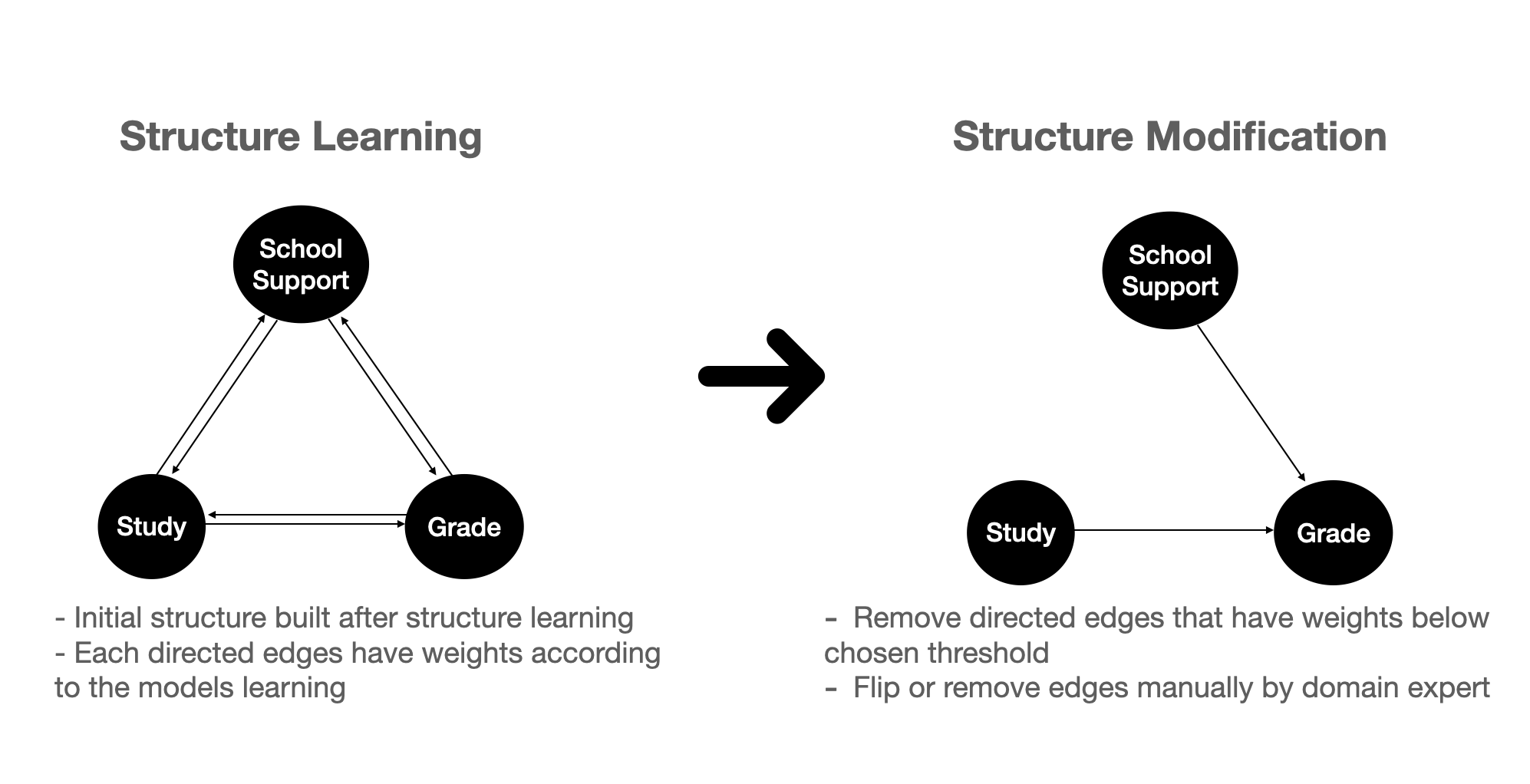
Figure 4 above shows the steps in building a bayesian network:

• First, we can use some algorithm (NOTEARS) to automatically build edges between our variables.
• As a consequence of the learning process, the edges have weights. Hence we can remove some edges that are below a certain threshold. This results in an initial causal structure build automatically from the algorithm.
• We can then further proceed to fix the causal structure by flipping, removing, or adding edges based on our domain knowledge.

What lies underneath bayesian network?

In the classical literature, bayesian networks are mostly either fully discrete or fully gaussian. This means that all the nodes in the graph are either discrete or continuous. The reason is because of closure properties: fully discrete allows us to model the conditional probability distribution with conditional table and they are all jointly multinomial random variable, whereas fully gaussian allows every operation (conditional, marginal, etc) to always result in another gaussian. There are other approaches where we use a non-parametric version of bayesian network which allows us to work flexibly with different types of distributions.

Parameter estimation in bayesian network

The structure tells us the causal relationships, and for each of these relationships, there is a distribution which tells us the probability of attaining a certain state given for any variable given the states of the parent node. In a fully discrete bayesian network, the size of the conditional probability table would be the number of states of current node multiplied by the parents state. This would be total parameter that we need to estimate from data. To estimate these parameters, one can use maximum likelihood estimation (usually just involves taking counts and fractions) which produces a point estimate or use bayesian estimation and allows us to put a prior belief on the estimate.

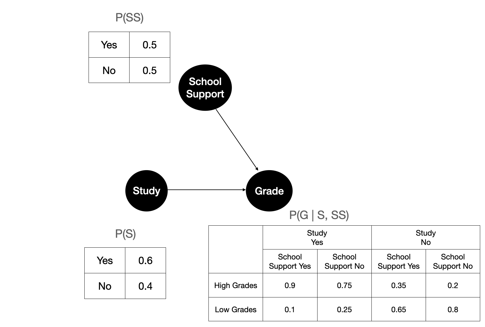
Figure 5 shows the illustration after fitting the parameters of our 3 variables on the observational data. Each node is governed by a conditional probability. If a variable does not have any parents, then it’s just its own probability.

The operation in bayesian network

With a bayesian network defined, one might ask: what can do with it? There are two operations that we can apply on a bayesian networks node: conditioning and intervention. Do note that conditioning is not always the same as the causal effect, that is why it is better to always do an intervention if we are able to and especially if we want to gain insight using the bayesian network.

Conditioning

Conditioning is an observational inference: having observed the data that we have, what would the probability of a certain variable be given that we observe some parents state. Since conditioning is observational, we can do conditioning between any arbitrary nodes without having to follow the directed edge (yes including between nodes that doesn’t have any directed arrows). Conditioning is usually done in a setting where one cannot do an intervention. In conditioning, we can have a non-causal correlation flowing from one node to another node if we are not careful, leading to an incorrect interpretation. In other words, conditioning between arbitrary nodes without regarding the causal effect might lead to a spurious correlation. Consider this case below:

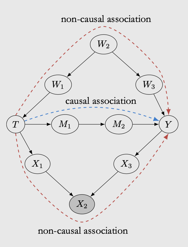
The true causal effect from treatment \(T\) to outcome \(Y\) flows through \(M1\) and \(M2\). However, in the case above there are two other paths in which non-causal correlation can flow from \(T\) to \(Y\):

• \(W1\), \(W2\), \(W3\)

• \(X1\), \(X2\), \(X3\)

The \(W\) path is known as confounder path. In bayesian network, confounder path can mess with the treatment effect because it affect how treatment \(T\) is assigned, making \(Y\) also affected. The only way to measure the treatment effect correctly in this case is by conditioning on all possible confounder. In the case of bayesian network, if we intervene on \(T\), then the non-causal association in the W path is automatically blocked. If we cannot do an intervention and would want to derive treatment effect from observational data, then the W path needs to be conditioned on, otherwise the non-causal association will render the causal effect incorrect. In the \(W\) path, conditioning on children of colliders (either \(W1\) or \(W3\)) also blocks the non-causal association, so it doesn’t have to be on the confounder node.

The \(X\) path is known as colliders. Contrary to the confounder, conditioning on the collider can make non-causal association flows through the path. We will not go into details but here is an excellent example of colliders. The idea is that if we have colliders, we should not apply conditioning on that variable as it can mess with our interpretation.

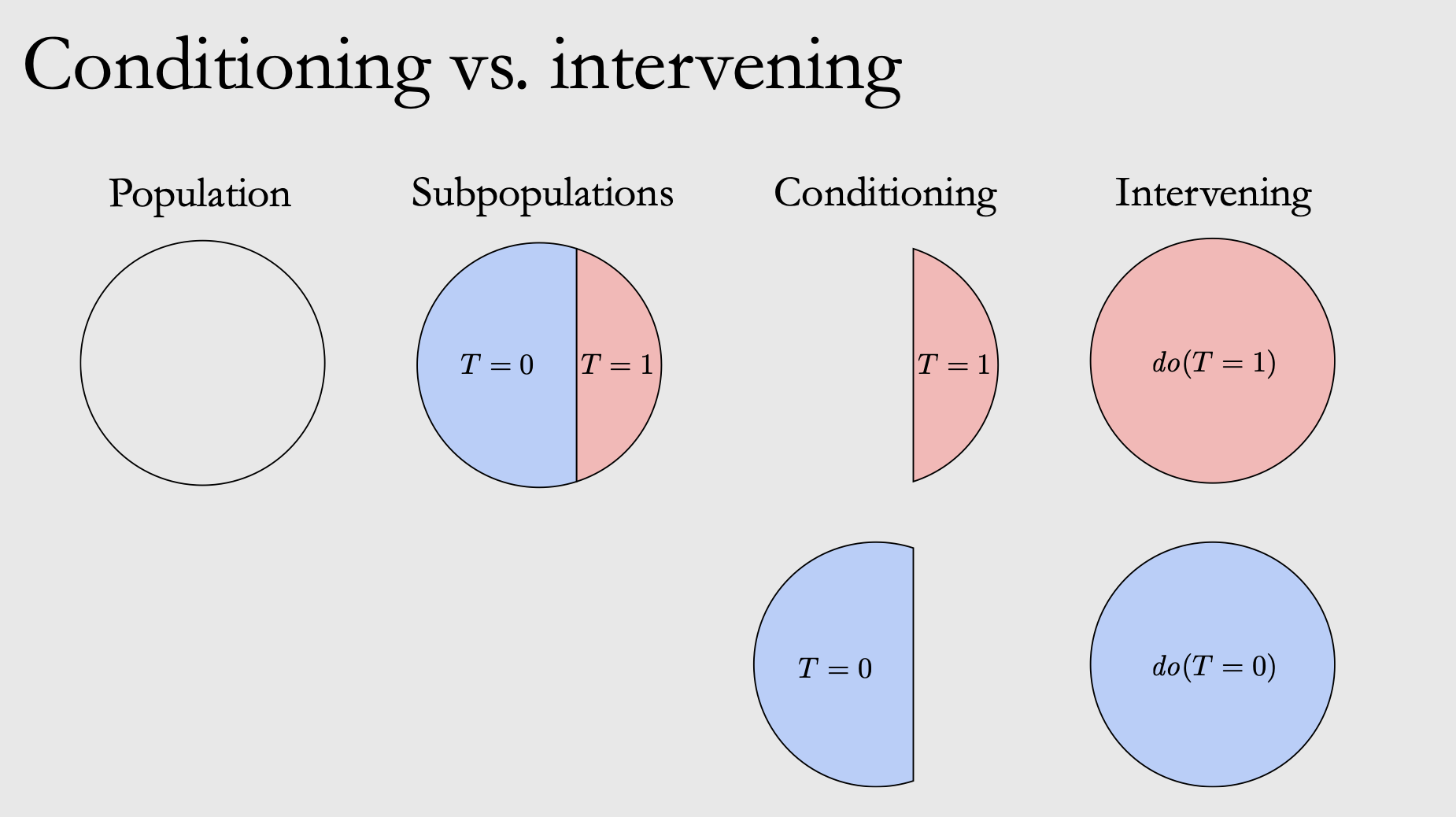
Intervention

To gain insight from our model, we want to query our model under different observation. With intervention, we can replace the probability distributions of a certain state. If this state has a children, then we can simulate what would have happened to the children marginal probability if we do an intervention to the node. Unlike conditioning, intervention on a node will only affect its children according to the causal direction. Figure 8 and 9 below shows how we can do an intervention to simulate the target variable.

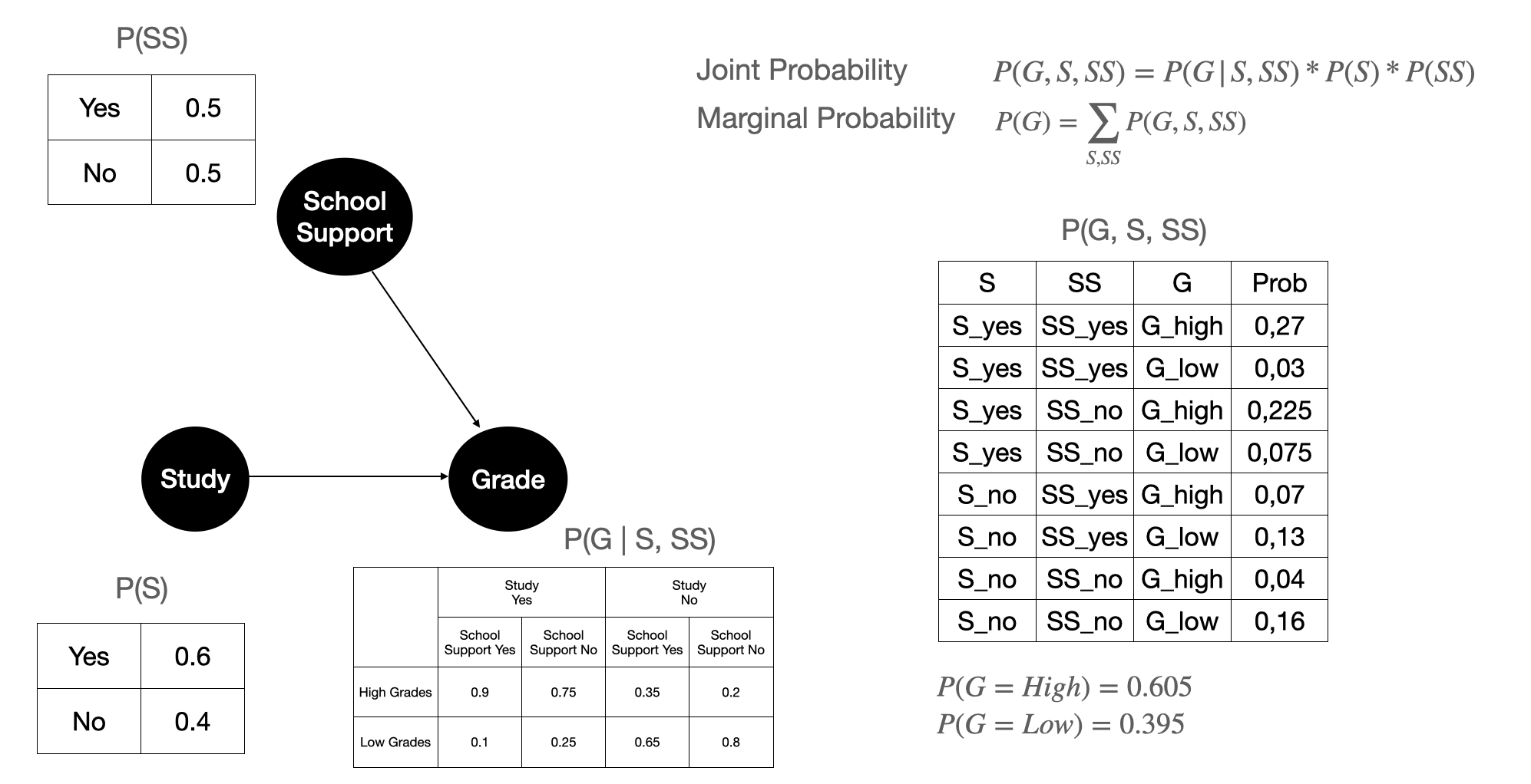
Figure 8 shows the calculation of the joint probability between Grade, Study, and School Support, and the marginal probability of Grade. Remember that \(P(S)\), \(P(SS)\), and \(P(G \mid S, SS)\) are calculated from data. These are the parameters that we estimated after we have the causal structure. With the estimated parameter and causal structure, we calculate the marginal probability of Grade. This is the marginal probability that we learn from data before we do any intervention.

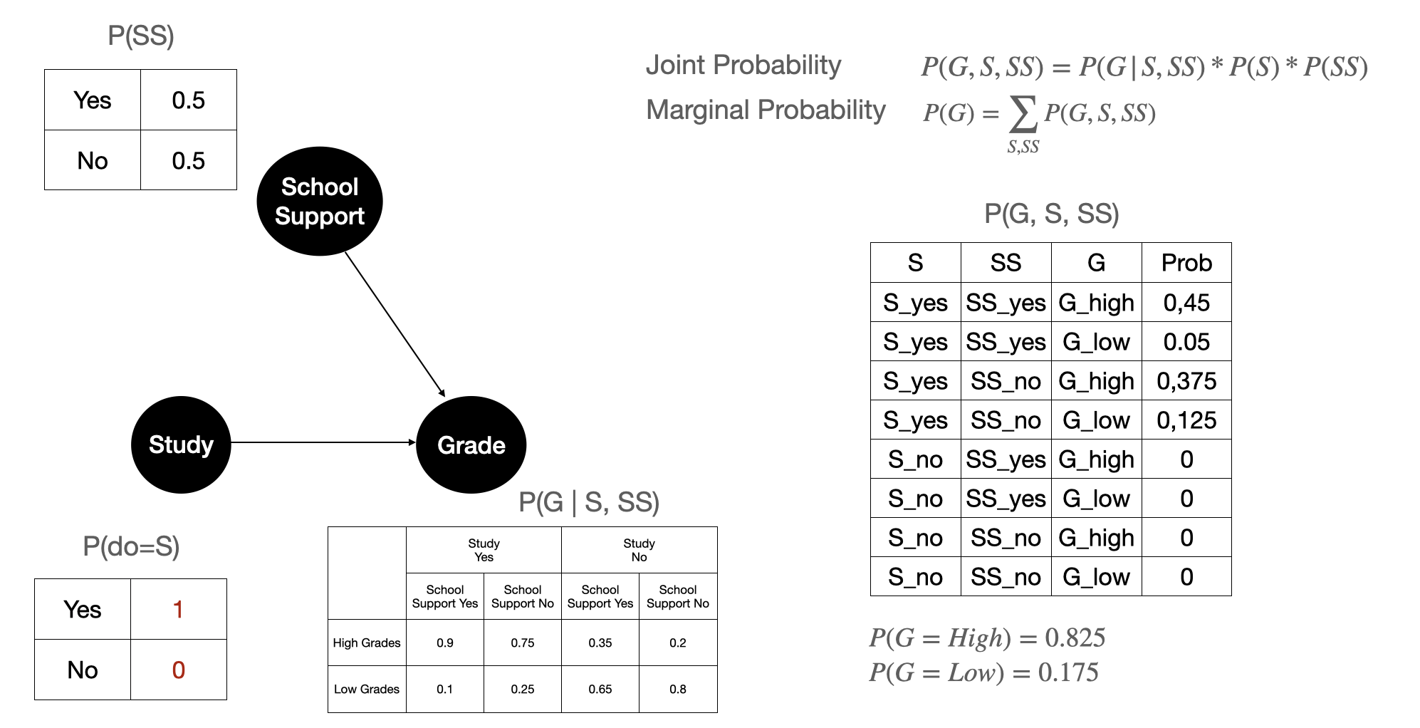
Figure 9 shows how it would look like to Grade variable if we do an intervention on Study. Here we force \(P(S)\) to hold a certain value: in plain English we can interpret this as forcing everyone to Study. We can see after intervening, the marginal probability of Grade from 0.605 to 0.875 on the marginal probability \(P(G=High)\). This means that we can assume that if we nudge students to study more then it would yield better grades that is good for the school.

Please note that when doing intervention, we assume that the change in the target variables marginal probability happens on the whole population. However, when we build the causal structure and fit the parameters for every variables, we do it on the observational data. So it’s important to make sure that we have enough data first. Ensuring that we have enough data is most commonly known as fulfilling the positivity/overlap assumption.

Recap and closing

In this post we cover structural causal model as a way to capture causal language. We have seen:

• Simpson’s paradox in a graph.
• Directed acyclic graph, especially bayesian network, as a structure to model both association and causation relationship between variables.
• How to build bayesian network given data.
• Condition and intervention as operations that we can apply in bayesian network.

Thanks for reading this post! Contact me on twitter for feedback @rezkaaufar