“Correlation does not imply causation”

You might hear this jargon everywhere since it is quite pervasive if you work in data science/machine learning. Also, you might have seen this image about spurious correlation:

But what does it mean, really? What does “correlation does not imply causation” really mean? Given a data \(X\) and a target variable \(Y\), can we estimate direct causal effect? If so, how can we know that we have modeled causation in a correct way? Is there a formal way to capture this English statement? Yes!

In causal inference, there are at least two formal ways to discuss causation: one is based on counterfactuals (or potential outcomes) and the other one is based on causal directed acyclic graph (or structural causal model). The latter involves Judea Pearl’s do-calculus. For the rest of this post I am going to use the former, which is the language of counterfactuals to draw the intuition. Okay, enough intro. The best way to start understanding why correlation \(\neq\) causation is to understand the simpson’s paradox.

Simpson’s paradox

Imagine we are developing a treatment for both men and women. We want to know the causal effect of the treatment. Specifically, we want to draw a conclusion from the treatment with the following possibility:

• Treatment is good for men (S1)
• Treatment is good for women (S2)
• Treatment is bad overall (S3)

Now, simpson’s paradox occurs when people equate probabilistic statements with the statements (S1), (S2), and (S3) above. How does the probabilistic statements look like? Consider the data below

From the table, we have treatment \(T\) that is binary (given and not given), feature (or covariate) \(X\) that is also binary (men and women) and the outcome \(Y\) that is also binary (working and not working). The numbers in the column is the sum of treatment that is working (\(Y=1\)). Consequently, we have the probabilistic interpretation as follows:

• \(P(Y=1 | T=1, X=1) = 0.15\) (Group 1)

• \(P(Y=1 | T=0, X=1) = 0.10\) (Group 2)

• \(P(Y=1 | T=1, X=0) = 0.30\) (Group 3)

• \(P(Y=1 | T=0, X=0) = 0.20\) (Group 4)

• \(P(Y=1 | T=1) = 0.16\) (Group 5)

• \(P(Y=1 | T=0) = 0.19\) (Group 6)

From the probabilistic interpretation above, we can derive three key probabilistic statements:

• \(P(Y=1 | T=1, X=1) - P(Y=1 | T=0, X=1) > 0\) (P1)

• \(P(Y=1 | T=1, X=0) - P(Y=1 | T=0, X=0) > 0\) (P2)

• \(P(Y=1 | T=1) - P(Y=1 | T=0) < 0\) (P3)

Remember: simpson’s paradox occur when people equate probabilistic statements (P1-P3) with the English statements (S1-S3). We see from the example above, all (P1), (P2), and (P3) are true. But in causal inference, it is NOT possible for (S1), (S2), and (S3) to all be true. If the treatment is good for both men and women (S1-S2), then it should not be possible that the overall treatment is bad (S3). But why does our observation says otherwise? Again, the error is in equating (P1-P3) with (S1-S3).

How does this happen then? Is it because of the sample size that is not comparable between groups? Well we can still have more or less the same sample size and still fall to simpson’s paradox (example). To understand why this is happening, we need to understand the effect of confounding variable.

Confounding variable

Let’s take a closer look at Table 1. Do you notice a pattern in the treatment assignment? You can see that the there are more treated men than those who doesn’t receive treatment. On the other hand, there are less treated women than those who doesn’t receive treatment. We might wonder: gender probably affects the treatment assignment, therefore there are more men who received treatment than women, which led to non-comparable groups formed between men and woman. In this case, gender is a confounding variable. Confounding variable is a common cause that is both affecting the treatment and the treatment outcome. Usually confounding variable is unobserved.

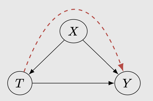
There is an information flow between the treatment to the outcome via the confounding variable, resulting in (P1-P3) to all be true. In this case, \(X\) is the confounding variable: the gender.

Correlation does not imply causation (in a formal way)

To capture the English statements (S1-S3) above, we use counterfactuals. We start by introducing \((Y1, Y0)\) where \(Y1\) is the outcome if one is treated and \(Y0\) is the outcome if one is not treated. We observe:

To put it simply, \(Y1\) denotes the outcome I WOULD observe if I WERE to take the treatment, \(Y0\) denotes the outcome I WOULD observe if I WERE to not take the treatment, whereas \(Y\) denotes the outcome that I do observe just in the observational data. In reality, we never observe \(Y1\) and \(Y0\) in the observational data on any person, that is why when we derive conclusion DIRECTLY from Y, we observe the simpson’s paradox. We’ll see more details regarding counterfactuals in the next section.

The correct translation of (S1-S3) is:

• \(P(Y1=1 | X=1) - P(Y0=1 |X=1) > 0\) (C1)

• \(P(Y1=1 | X=0) - P(Y0=1 |X=0) > 0\) (C2)

• \(P(Y1=1) - P(Y0=1) < 0\) (C3)

These three statements cannot be all true. If the first two statements hold, then:

This is why if the treatment is good for both men and women (S1-S2) , then it is not possible that the overall treatment is bad (S3). In summary:

• (C1) = (E1) \(\neq\) (P1)
• (C2) = (E2) \(\neq\) (P2)
• (C3) = (E3) \(\neq\) (P3)

and (E3) cannot be true if (E1) and/or (E2) hold. In general, we have:

In other words, correlation (left hand side) does not imply causation (right hand side). The left hand side can also be called the probabilistic quantity and the right hand side can be called causal quantity.

Counterfactuals

I mentioned above that in order to capture the causal statements, we can use counterfactuals (or potential outcome). But what does it mean? In our binary treatment example, counterfactuals are the outcomes that we could have observed if we can give treatment and not give treatment to a person simultaneously. Ideally, to measure the true causal effect, we would want to put everyone in the population in both the treatment group and control group(s). Consider the men group in Table 1: the true causal effect is the difference between all 1450 people for the treatment group and all 1450 people for the control group. In other words, we want both the outcome for treatment and no treatment to be available for everyone. But in this case (and almost always) the counterfactuals cannot be observed, hence we take the naive difference between n=1400 and n=50.

So how do we derive the correct causal effect then? How can we get \(Y1\) and \(Y0\) so that we can reliably say that my treatment has an effect? Do we have to fill in all the counterfactuals so that we have the same number of instances between groups? As far as I understand, there are two ways we can derive causal effect reliably:

• Randomized controlled trial (or AB Test).
• Conditioning on all possible confounding variables.

The former usually does not involve in filling all the counterfactuals (which we’ll see more below). The latter approach is used in a situation where it is almost impossible to do randomized controlled trials (e.g. telling non-smoker to smoke to determine the causal effect of smoking to impotence). The latter is also mostly used on observational data. Furthermore, in the latter case we can take it further by filling the counterfactuals to get the best causal effect estimate.

Randomized controlled trials

RCT/AB test removes the effects of confounding to the treatment. Directed edge from \(X->T\) is removed.

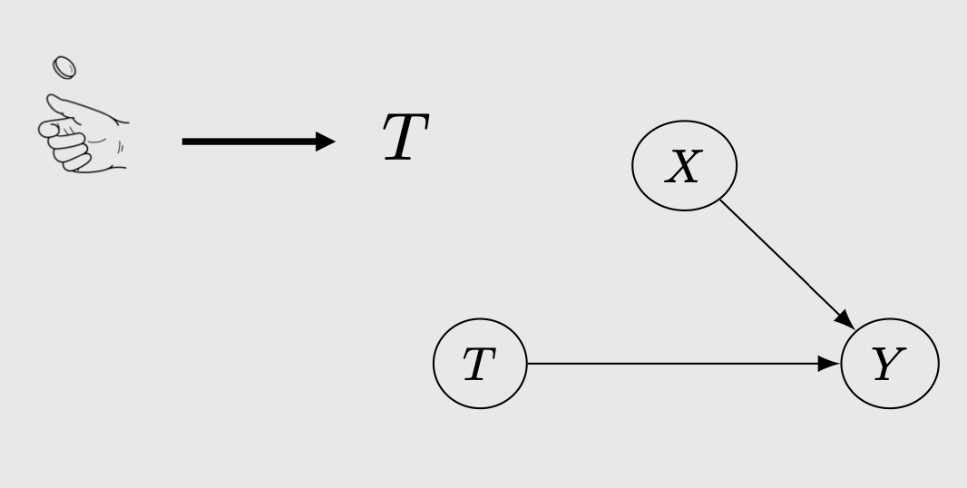
This means that the treatment assignments are now purely random. Consequently, this makes \(T\) independent of \((Y1, Y0)\), or in other words, the treatment does not affect the potential outcome anymore. Note the difference: treatment \(T\) still affect the actual outcome \(Y\) but the treatment DOES NOT affect the potential outcome \(Y1\), \(Y0\). For more intuition regarding this I highly recommend checking out Brady Neal’s causal inference course. With the independence, we have

hence we can assume that the probabilistic quantity (P1-P1) is now the same as the causal quantity (C1-C3). Therefore, we can derive the causal effect directly from the probabilistic quantity and do your statistical test to determine whether it is significant (the usual AB Test). In RCT, afaik, we can sort of trust the outcome because of the randomized treatment assignment without having to approximate the counterfactuals.

Observational data

In the case of most observational data, where the treatment assignment is not random, we can only recover the causal effect by CONDITIONING on all possible confounding variables.

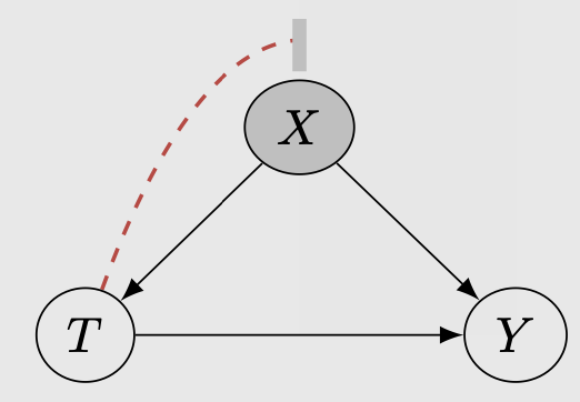
Essentially, we want the independence between \(T\) and \((Y1, Y0)\) to happen here but we do this via conditioning on the confounding variables. We have:

This condition reduces the causal effect into a probabilisitic quantity. In the above example, if we assume that gender is our confounding variable, conditioning on it would yield:

\(P(Y1 = 1) = \sum_x P(Y = 1 | T = 1, X=x) P(X=x)\) , where there is only one \(x\), namely gender

Now, to further calculate the causal effect in a non-randomized observational data, it is common to approximate the unobserved counterfactuals with a prediction. In the men group above, we can train a model to predict the unobserved counterfactuals to fill the missing data points (so we have treated men n=1450, not treated men n=1450) and then predict the average treatment effect between the two groups. There are many ways to create this approximate causal model and they usually involve a lot of assumption. For more details I highly recommend to also check this MIT lecture notes. The most important assumption is of no unmeasured confounders, which only holds when we observe all possible variables that influence both treatment decisions and potential outcomes. In reality, one has to consult with a domain expert to make sure that all variables that influence treatments and potential outcomes are observed.

Application in industry

This is something that I am curious about, but unfortunately I haven’t found the opportunity that allowed me to implement causal inference in a work setting. So I can’t speak from experience. Here are some examples of causal inference that I know can be beneficial in industry:

Uplift modeling

It is aimed at quantifying the treatment effect and identifying the characteristics of individuals most likely to benefit from the benefit. With this information, one thing we can do is to better choose individuals for the next cycle. The characteristics identification is essentially a prediction of counterfactuals for a customer in an experiment setting. Afaik, uplift can also be used to generate demand by giving user more targeted coupons or voucher. Uplift modeling can be used together with AB Test (offline) or multi armed bandit (online).

Causal DAGs for forecasting

I do not know much about this since this is probably still a new field. One example that I know of is from Lyft (check this talk from Sean Taylor). At Lyft, they create a causal DAGs with prior experimental evidence to model the causal effect of things. In the causal DAGs, there are:

• pure parent nodes that they control (price level, how much we spend on driver incentives)
• outcome nodes that they monitor (marketplace outcome, things that happen)
• pure parent nodes that they do not control (how many people request driver organically)

They seem to have another model (like policy variables) that produces plan. This plan is then inserted into the structural causal model to sort of simulate what would happen in the outcome nodes.

Sean mentioned that in the business context, they need to estimate the effects of choices they make, and making those choices are causes in both the causality and causal inference senses. The estimates produced by their causal models are inputs to decision problems. Ultimately, they still need to do some decision-making (either by humans or algorithmically) that is informed by their models. I think that they cover more complex interventions involving multiple treatments and outcomes.

If you know any other implementation of causal inference in industry, please do let me know!

Recap and closing

What this post covered:

• Correlation vs causation in a formal way.
• Counterfactuals as a causal language to capture causal effect correctly. By introducing potential outcomes \((Y1, Y0)\) we see where the failure is.
• RCT and conditioning on confounding variables as a way to reliably calculate causal effect in an experiment.

What this post doesn’t cover:

• List of assumptions that need to hold for the counterfactuals to work.
• Structural causal model (Pearl): another causal language to describe and capture causal effect.

Thanks for reading this post! I am a noob in causal inference so please do inform me if there is an error or mistake on twitter @rezkaaufar