Lexical match in a search engine retrieval
Have you ever wondered how search engine works? How can it match a query with millions of documents super fast and return them to the users?
In this post, we are going to look at one of the most fundamental technique in search retrieval: lexical match.

Figure 1: Query and document..
Retrieval
In retrieval, we want to return a smaller pool of documents from the huge pools given a query. Imagine that in a system where we have millions of documents and we want to retrieve a subset of documents that are relevant to a given query. The subset essentially is a smaller pool of documents that we want to do further processing on. The goal of the system is to reduce the number of document candidates that can potentially be of interest according to a given query.
There are many techniques to do retrieval, and one of the oldest and battle-tested technique is to use lexical match. The key point is retrieval needs to be fast. In Big-O notation, we want the retrieval to have a time complexity in $\mathcal{O}(1)$ or at most in $\mathcal{O}(\log N)$. Higher time complexity yields to slow and unpleasant experience for users.
Retrieval with inverted index
For the sake of simplicity, let’s assume that the query and documents that we have are of string types. To do retrieval fast, we create an inverted index which stores every unique token (vocabulary) that can be found in the document pool and points to document subset containing this token.
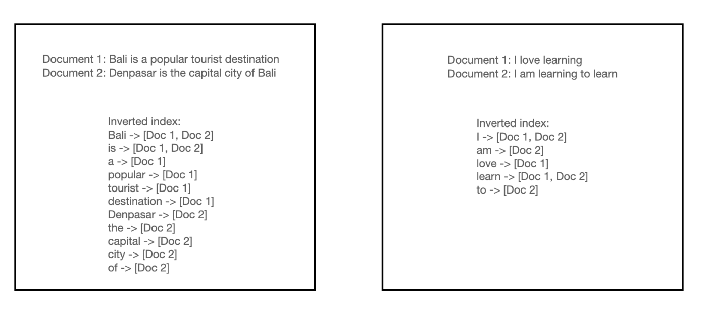
Figure 2: Inverted index.
So instead of doing a string match for every query term to the document term, we can directly access the index to return the list of documents of matched query in $\mathcal{O}(1)$ time complexity.
In popular search libraries such as Elasticsearch, we can make further adjustments on the query and documents preprocessing and on how to define a match between a query and a document. These two techniques is going to affect how the inverted index is built and how the documents are retrieved.
We can preprocess both the query and the documents using variety of techniques. For example, we can stem words to only include base word, tokenize word using different delimiters (not only using the space as the delimiter), remove stop words, and many more.
For a match between a query and a document, we can determine whether we want full match of all query term, partial match only, or any other heuristics. Full match means that all query terms must be present in the document. Partial match means that at least one query term must be present in the document. These heuristics give you some control on which criteria you want the documents to be returned.
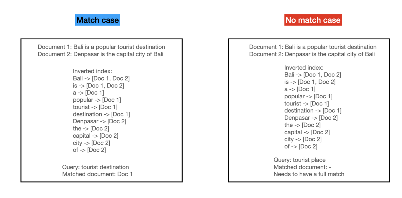
Figure 3: Inverted index match case.
Assigning score to the retrieved documents
We need to assign a score to each of the retrieved documents so that we can get the rank from the most relevant items the least relevant items with respect to the query term. There are many ways to assign score to each retrieved documents, from the older approach like tf-idf and bm25 to the more neural network approach. In this post, we’ll take a look at tf-idf.
TF-IDF scoring
For the following illustration, we have 4 documents in total with vocabulary size of 8: “blue, bright, can, see, shining, sky, sun, today”.
As the name suggest, there are two components in tf-idf: term frequency - inverse document frequency.
Given a word $t$ and document $d$, term frequency $f_{t,d}$ is simply the number of times each word $t$ appeared in document $d$. We can also calculate $tf(t,d)$ which is the normalized term frequency by dividing the term frequency by the total number of words in the document.

Figure 4: Term frequency.
Inverse document frequency measures how rare $t$ is across the corpus $D$. Given $N = D$ as the total number of documents in the corpus and $n_t$ as the number of documents having $t$, the $idf(t,D)$ can be calculated as:

Figure 5: Inverse document frequency.
Given the tf and idf, we can multiply them together to get the tf-idf score.
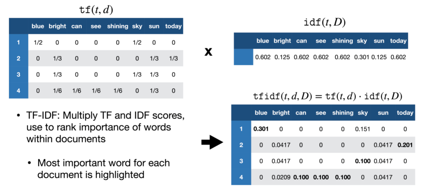
Figure 6: tf-idf final score.
Calculate tf-idf score for new query
Say that your system is running in production, how does it work when you have new query coming in? For term frequency (tf) we need to calculate it real-time. For idf, we can just use the precomputed idf that we store somewhere in the system. See the illustration below:
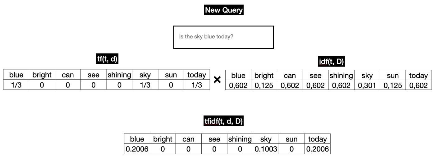
Figure 7: Reranked list with tf-idf score.
Once we have the tf-idf vector, we still need to calculate the similarity between the query and the matched product tf-idf vectors. The tf-idf vector of the matched product is precomputed, so we do not have to recompute this. For the similarity metric, most library uses cosine similarity. This step is $\mathcal{O}(m \cdot k)$ where $m$ is the number of matched products and $k$ is the dimension of the tf-idf vector.
In reality though, most of the values are zero because a single document or query only uses a tiny fraction of the total vocabulary. So although the textbook definition of a tf-idf vector is a vector of size $k$ vocabulary, in practice it is stored as a sparse vector. Instead of a fixed-size array of $k$ vocabulary size, we store a Dictionary/Map of only the non-zero indices.
Query: {term_id_42: 0.5, term_id_889: 0.8}
Document: {term_id_12: 0.1, term_id_42: 0.4}
So when calculating the cosine similarity, we only need to iterate through the non-zero indices of the query vector. In this case, we only need to iterate through the term_id_42 and term_id_889. We don’t need to iterate through the term_id_12 because it is not present in the query vector.
Example Walkthrough:
Query: {42: 0.5, 889: 0.8}
Document: {12: 0.1, 42: 0.4}

1. Look at Query Key 42: It exists in the Document. 42 has a value of 0.5 in the query and 0.4 in the document.
    0.5 * 0.4 = 0.2
    score = 0.2

2. Look at Query Key 889: It does not exist in the Document.
    skip

Final Score: 0.2
Appendix
Image source for Figure 4,5 and 6.