Things to look out for when running CUPED

March 15, 2026 · 9 min read · statisticsexperimentation

We have a new feature that we want to test. We calculate sample sizes required and the stakeholders are not happy with the duration it took to run the test. They said we need to go faster with the decision and we can’t afford to run an AB test for this long. We go back to the drawing board and try to find a way to reduce the sample size. Can we reduce the sample size required but still maintain the same power?

One of the most common method to reduce variance in an AB test is by using CUPED (Controlled-experiment Using Pre-Experiment Data). CUPED is a variance reduction technique that can be used to reduce the variance of an estimator by using a control variate.

In this post, we are not going to go through the math behind CUPED. Instead, we are going to go through the things to look out for when running CUPED. We’ll start with a brief introduction on what CUPED is and how it works. And then we go into the considerations that we need to take into account when running CUPED.

Please note that the approach that is described in this post is based on my interpretation of the original CUPED paper. It is possible that there are other ways to implement CUPED and it is possible that my interpretation is incorrect. Please refer to the original paper for more details.

CUPED background

The idea of CUPED is that we can use historical data to neutralize pre-existing noise. Let’s say we have a metric that we measure $Y_1$ that we observe after we start the experiment. The goal is to find a historical pre-experiment data $Y_0$ that has a strong correlation with $Y_1$ to adjust the observed $Y_1$. In practice, $Y_0$ needs to be:

as correlated as possible with $Y_1$ to maximize the variance reduction
independent of the treatment assignment.

In the original CUPED paper, the authors suggest to use the pre-treatment outcome $Y_0$. In other words, the unit of $Y_0$ has to be the same as $Y_1$.

To illustrate, lets say our analysis unit is a user. We want to measure the users’ conversions $Y_1$ by giving a discount voucher $T$ as our treatment. We can use the users’ conversions $Y_0$ before the experiment starts as our control variate.

What we do is:

Regress $Y_1$ on $Y_0$ and estimate the coefficient $\hat{\theta}$.
Compute $Y_{1}^{cuped} = Y_1 - \hat{\theta} Y_0$ for each unit.
Compute the difference of $Y_{1}^{cuped}$ between treatment and control group.

Here is how it looks in python code:

theta = smf.ols('conversion_post ~ conversion_pre', data=df).fit().params[1]

df['conversion_cuped'] = df['conversion_post'] - theta * (df['conversion_pre'] - np.mean(df['conversion_pre']))

smf.ols('conversion_cuped ~ discount_voucher', data=df).fit().summary().tables[1]

What we will observe is that the output of the second regression will have a much smaller standard error compared to the first regression. This is because CUPED has reduced the variance of the estimator. For more illustrative example, you can refer to this notebook.

Do we even observe $Y_1$ before the experiment starts?

Remember that when calculating sample size, we are using the variance of the estimator. With CUPED, we want to reduce the variance of the estimator before the experiment starts. The first thing that you might be wondering is that do we even observe $Y_1$ before the experiment starts to calculate CUPED? In reality, we only observe $Y_1$ after the experiment starts. So then how do we do the regression to get $\hat{\theta}$ before the experiment to further calculate $Y_1^{cuped}$?

One approach that we can do is to split our historical data into two parts as if we are running an experiment. Let’s say we take the last 4 weeks of historical data, we can use the first 2 weeks as our pre-experiment data (i.e., $Y_0$) and our second 2 weeks as our experiment period (i.e., $Y_1$). We can then calculate $\hat{\theta}_{hist}$ using the pre-experiment data by running the first regression:

\[Y_1 \sim Y_0\]

where $Y_0$ is the pre-experiment data and $Y_1$ is the experiment data. We can then use the $\hat{\theta}_{hist}$ to adjust our required sample sizes:

\[N_{new} = N_{old} \times (1 - \hat{\theta}_{hist})^2\]

where $N_{old}$ is the original sample size calculated using the usual power analysis formula and $N_{new}$ is the new sample size required to achieve the same power with CUPED.

The risk of this approach is that the historical correlation coefficient $\hat{\theta}_{hist}$ is not guaranteed to be perfectly correct for the live experiment. It is strictly a proxy used to guess the required sample size. This approach relies on the assumption that the analysis unit behavior is consistent over time. If the analysis unit behavior changes between the historical period and the live experiment, then the estimated $\hat{\theta}_{hist}$ could be incorrect. Therefore, the required sample size calculated using $\hat{\theta}_{hist}$ could be incorrect as well. For example, lets say our sample size calculation using $\hat{\theta}_{hist}$ is 2 weeks but it actually needs 4 weeks because the real variance reduction was weaker than expected.

To improve the accuracy of the required sample size calculation, we can instead run CUPED calculation frequently after we start the experiment using the actual $Y_1$. Once we begin to get the actual $Y_1$, we stop using the historical estimate and recalculate the sample size required using the actual $\hat{\theta}_{actual}$.

Let’s say we need 4 weeks of data to run the experiment ($N_{original} = 4$). With the historical correlation coefficient, we calculated the required sample size to be 2 weeks ($N_{historical} = 2$). Every day after the experiment starts, we can calculate the actual $\hat{\theta}_{actual}$ and observe the variance reduction. The variance reduction is going to fluctuate in the short term but it will eventually converge to the true variance reduction. This is illustrated in this image below:

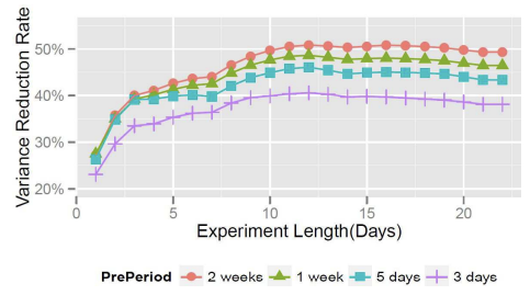
Figure 1: Variance reduction over time from Deng et al (2013)

Once it reaches a stable point, we can recalculate the required sample. In the example above, we can see that the variance reduction has stabilized over the last 5 days at day 15. Hence, at day 15, we can then re-calculate the required sample size. Let’s say, at day 15, the variance reduction applied to the original sample size ($N_{original} = 4$) is to be 3 weeks ($N_{new} = 3$). Then we can run let the experiment run until the 21st day and stop there instead of waiting until the 28th day according to the original sample size calculation.

To recap our illustration:

Original sample size calculation without CUPED: 28 days, 4 weeks
Required sample size calculation with CUPED historical: 14 days, 2 weeks - overestimated variance reduction
Required sample size calculation with CUPED actual at day 15 once it stabilized: 21 days, 3 weeks
Stop experiment at day 21 instead of day 28

The main takeaway from me is that it is better to just run CUPED frequently with the actual $Y_1$ instead of using the historical estimate as it is more accurate. Once we observe our variance reduction to be stable, we can then re-calculate the required sample size and stop the experiment at the right time.

The only caveat here is that we cannot run CUPED before the experiment starts, whereas with the historical estimate, we can run CUPED before the experiment starts. Here, we have to wait until the experiment starts to get the actual $Y_1$. So we let the experiment runs first with the original sample size calculation and then we run CUPED with the actual $Y_1$ to shorten the duration of the experiment.

My analysis unit does not have consistent pre-experiment identity

Another thing to note with CUPED is that it requires the analysis unit to have a consistent pre-experiment identity. For example: in an online retail platform, if the analysis unit is at order level, then it is not possible to have a consistent pre-experiment identity. An order can be created in the pre-experiment period and the same order is not going to be available in the experiment period. An order is a transient unit, not a persistent unit.

One possible solution for this is to map the transient analysis unit to a persistent unit. The original paper by Deng et al (2013) discussed this under the Handling Non-User Metrics section, where they talk about the challenges when our analysis unit is different than our randomization unit. In their case, the randomization unit is at user level, but the analysis unit is at page level. They proposed delta method to produce correct estimate of variance that takes into account the correlation of pages from the same users. For interested readers, you can refer to their paper for more details. My interpretation is that with this approach, the goal is to link the transient unit (order) to a persistent entity (user, merchant, or cookie) and use that entity’s history as the covariate for the order.

Another possible solution is to use CUPAC, which stands for Control Using Predictions as Covariates. With CUPAC, we can build a machine learning model that takes in multiple input features to create a predicted $Y_{pre}$ that can be utilized as a covariate for CUPED calculation for the analysis unit after the experiment starts.

Here is my interpretation of the approach:

Assume pre-experiment we have user 1 with order 1, 2, 3, 4 and during the experiment we have user 2 with order 5, 6, 7, 8.
In this scenario, there is no way we can find a covariate ($Y_{pre}$) on the order 5, 6, 7, 8 as order is a transient unit.
With CUPAC, we can train CUPAC model using order 1, 2, 3, 4 to predict $Y_{pre}$ with input features. After the experiment start, we can use our trained CUPAC model to predict $\hat{Y}_{pre}$ for order 5, 6, 7, 8 given the input features.
Now for order 5, 6, 7, 8, we can use $\hat{Y}_{pre}$ as the covariate to adjust the observed $Y_1$ that can be used for CUPED calculation.
Here, our CUPAC model will be on order level, which is the analysis unit level, but the input features we use for CUPAC model can come from different granularity. Using ML model essentially transforms the input features into something that can be matched between pre-experiment and post-experiment.

The only thing to note with CUPAC is that the input features used to train the ML model needs to be invariant to the experiment. The attributes that the treatment cannot change.

Also note that even with CUPAC, we are still faced with the same issue above, where we need to wait until the experiment starts to get the actual $Y_1$ to be able to calculate our variance reduction.