How to interpret confidence intervals (correctly)

January 18, 2026 · 3 min read · stats

Confidence intervals

Confidence interval is a range of values that is likely to contain an unknown population parameter. If we were to repeat an experiment or a sampling process many times and calculate a confidence interval each time, 95% of those generated intervals would contain the true population parameter.

Here we visualize our confidence interval when we sample multiple times from a true population. The true population is a normal distribution with mean 100 and standard deviation of 15.

np.random.seed(42)  
pop_mean = 100      # True population mean
pop_std = 15       # True population standard deviation
n_samples = 50      # Number of times we draw a sample
confidence = 0.95   # 95% Confidence Level

Here is the result of our confidence interval visualization using 30 sample size:

Small Sample CI

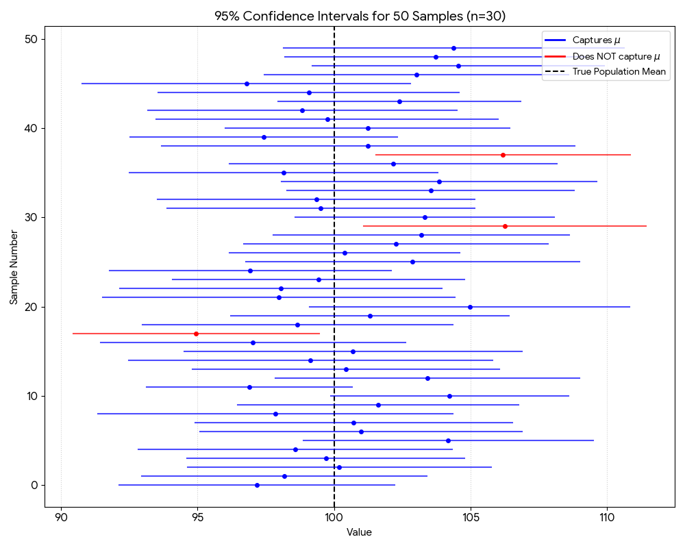
Figure 1: Confidence Interval with small sample size

We can see that of all the 50 sampling process, we have 3 confidence interval that does not contain the true population mean. This is in line with the 95% confidence level, where we expect 5% of the intervals to not contain the true population parameter.

Here we look at the result of our confidence interval visualization using 100 sample size:

Large Sample CI

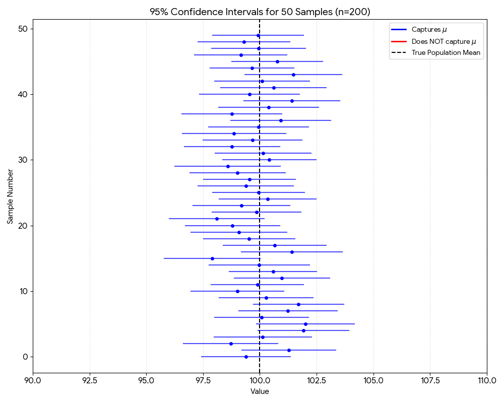
Figure 2: Confidence Interval with large sample size

With larger sample size, we expect to have more confidence intervals that contain the true population parameter. This is because larger sample size provides more information about the population, leading to more accurate estimates of the population parameter.

In the real world, we almost never have the luxury of repeating an experiment multiple times to see the distribution. We get one shot, one dataset, and one set of results. We can then turn to the Central Limit Theorem (CLT) to treat our single experiment as if it were part of that multiple sampling process. The Central Limit Theorem (CLT) states that the distribution of sample means will approach a normal distribution as the sample size increases, regardless of the shape of the population distribution. With the assumption that our single experiment is “typical” and not one of the rare outliers, we can use the CLT to construct a confidence interval for our population parameter and further do hypothesis testing from it.

Confidence intervals in linear regression

When doing linear regression, we also got confidence intervals and standard deviation for our estimated parameters. The standard deviation is calculated as such:

\[\hat{\sigma}^2 = \frac{\sum (y_i - \hat{y}_i)^2}{n - k}\] \[\text{Var}(\hat{\beta}) = \hat{\sigma}^2 (X^T X)^{-1}\] \[SE(\hat{\beta}_j) = \sqrt{\text{Var}(\hat{\beta}_j)}\]

where $\hat{\sigma}^2$ is the residual variance of the error term, $X$ is the independent variables, and $k$ is the number of parameters in the model.

Now, how can we interpret confidence intervals and standard deviation in linear regression?

For confidence intervals, this essentially means that if we were to fit a line many times, we can expect that 95% of the confidence interval contain the true parameter. For standard deviation, the theory behind it is also the same: if we took many different samples and fit a line to each, how much would the slope of that line vary?

Imagine the “true” relationship between two variables is a fixed, invisible line: $y = 5x + 2$. In the real world, we never see this line; we only see noisy data points scattered around it.

Sample 1: We collect 100 data points and fit a line. The slope estimate is $5.2$, and the 95% CI is [4.8, 5.6]. (This interval contains the true value of 5). The standard deviation of the slope is $0.4$.
Sample 2: We collect another 100 points. The slope is $4.9$, and the CI is [4.5, 5.3]. (This interval also contains 5). The standard deviation of the slope is $0.3$.
Sample 100: We collect 100 more points. This time, by pure random chance, we got a “weird” sample. The slope is $6.1$ and the CI is [5.7, 6.5]. (This interval misses the true value of 5). The standard deviation of the slope is $0.5$.

If we did this forever, 95% of those calculated brackets would successfully “capture” that true value of 5.

Here is the visualization of the confidence interval for the slope of the line:

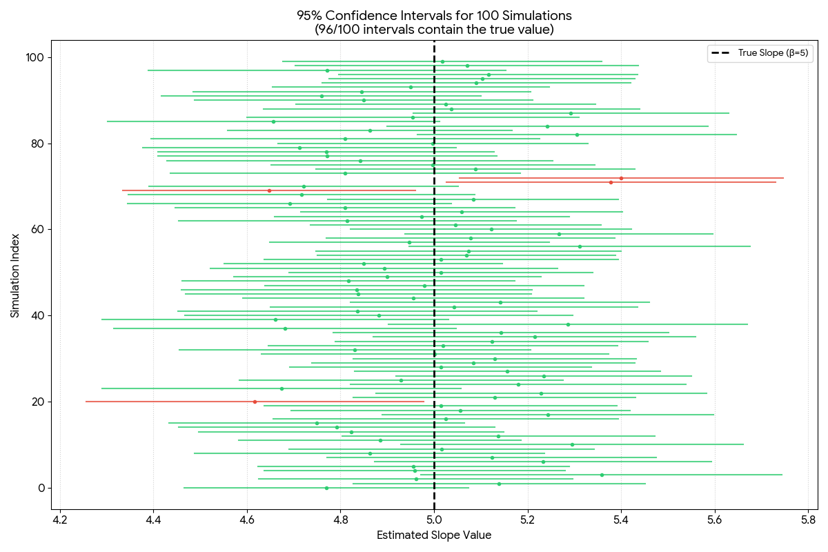
Figure 3: Confidence Interval for the slope of the line

Another thing to point is that in linear regression, we can view the parameter as the mean change in $Y$ for a unit change in $X$. So the mean of the distribution is here is bidimensional whereas the mean of the distribution in the previous example is unidimensional.