Non-compliance issue in an AB test
In a recent AB test that I did, I did the usual calculation of sample size, power, alpha, and MDE. At the end of the test, the test result was statistically significant. However, I then realized that some units in the treatment group were not actually doing the treatment. They were given the treatment but not all of them actually did it. This is a compliance issue that we need to address.
Non-compliance issue makes your test underpowered
We first looked at the average treatment effect between the treatment group and control group:
smf.ols('conversion ~ treatment', data=df).fit().summary()
The test result turn out to be statistically significant. But, given not all of the units in the treatment group actually did the treatment, our test is actually underpowered. Now what does this mean?
During the sample size calculation, when we set an initial Minimum Detectable Effect (MDE), we are defining the smallest “signal” we want to be able to see through the “noise” (variance) of your data. However, this rests under the assumption that all the treatment unit are actually the treated unit. In a non-compliance case, only a fraction of our treatment unit are actually the treated unit. Because of this non-compliers, the effect we actually observe in our dashboard is smaller than the true effect on the unit that actually did the treatment. The observed effect goes by the name of Intention-to-Treat (ITT) effect, while the true effect on the unit that actually did the treatment goes by the name of Local Average Treatment Effect (LATE).
Hence for our MDE to be valid, we need to adjust it based on the compliance rate. Assume for this post, our compliance rate is 60%.
mde_target = 0.02      # The MDE that we set, targeted for compliers
compliance = 0.6       # 60% compliance rate
true_itt = mde_target * compliance  # actual effect size: 1.2% ITT lift
So in our case, when we set our MDE to 2%, this is an MDE for the compliers. For the whole treatment group (or the ITT), we are actually targeting for 1.2% ITT lift. Hence the sample size we calculated is supposed to be done using the 1.2% ITT lift, not the 2% MDE.
Below is the thing we need to calculate for our sample size calculation:
sigma = 0.2 # Standard deviation of your metric
alpha = 0.05
target_power = 0.8

# Z-scores
z_alpha = stats.norm.ppf(1 - alpha/2)
z_beta = stats.norm.ppf(target_power)

# Sample Size Calculations
n_wrong = int(2 * (sigma**2) * (z_alpha + z_beta)**2 / (mde**2))
n_correct = int(n_wrong / (compliance**2))

se_diff_wrong = np.sqrt(2 * sigma**2 / n_wrong)
se_diff_correct = np.sqrt(2 * sigma**2 / n_correct)

threshold_wrong = z_alpha * se_diff_wrong
threshold_correct = z_alpha * se_diff_correct
And here is how our distribution of mean difference looked like when we use the wrong sample size and the correct sample size:
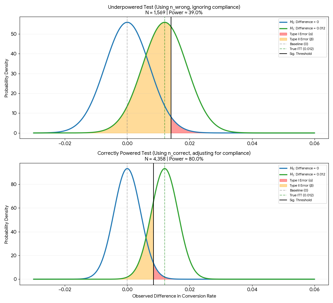 Figure 1: Comparison of mean difference distribution when using wrong and correct sample size
Notice that here we are not using the MDE as our H1 mean. Instead, we are using the true ITT lift as our H1 mean. This is because we are interested in the effect on the whole treatment group, not just the compliers.
From the image above, we can see that if we use the wrong sample size, the distribution is much wider. The orange area is massive, and the significance threshold (threshold_wrong) is to the right of the H1 mean. This means that even if we observe the True ITT during our test, we would fail to reject the null hypothesis. In this situation, we are more likely to make a Type II error (false negative).
Once we use the correct sample size by applying the $1/c^2$ correction (common correction on non-compliance issue), the distribution becomes narrower. The significance threshold shifts to the left (threshold_correct) and we can see that we now have 80% power to detect the treatment effect.
Now back to my original AB test, our test was underpowered but we still got a statistically significant result. Does this mean that we can conclude that the treatment is effective? Not at all. We just got lucky. If our “true” effect is actually 0.012, our data had to “get lucky” and swing into that thin green tail on the right side of the signicant threshold to be significant. This is the definition of Magnitude Error: our result is significant only because it is an outlier that is larger than the true average.
We can also do some simulation to check the average of the significant results from both the wrong and correct sample size test.
# Simulation
n_sims = 50000

results_wrong = np.random.normal(true_itt, se_diff_wrong, n_sims)
results_correct = np.random.normal(true_itt, se_diff_correct, n_sims)

# Determine significance (two-tailed)
sig_wrong = np.abs(results_wrong / se_diff_wrong) > z_alpha
sig_correct = np.abs(results_correct / se_diff_correct) > z_alpha
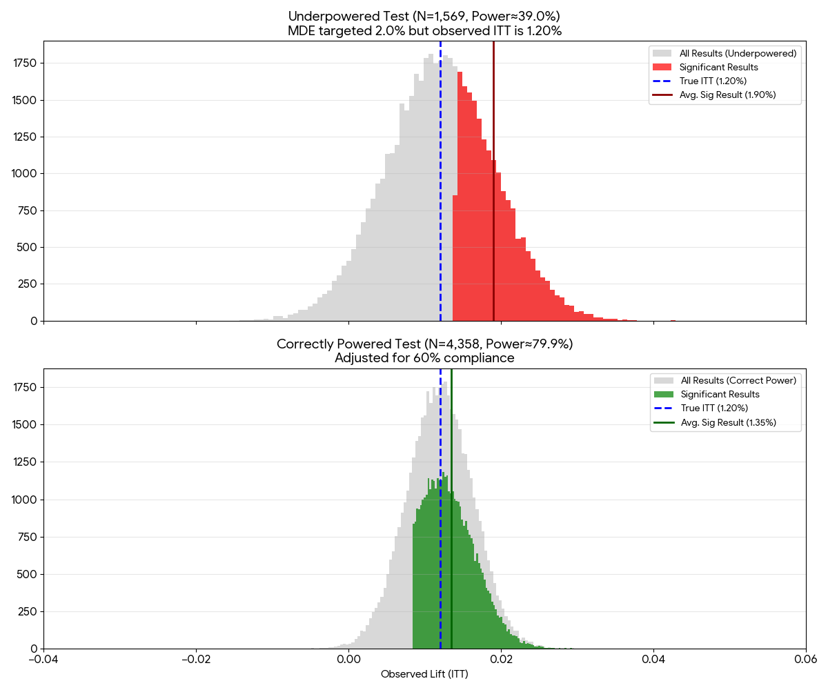 Figure 2: Simulation of the observed effect when using wrong and correct sample size
We can see that in our underpowered test, our average significant result is 1.90, closer to our original MDE of 2%. Whereas in the correct sample size test, our average significant result is 1.20, closer to our true ITT lift of 1.2%. This is inline with our previous analysis where the significance threshold of the underpowered test is higher than the significane threshold of the correct sample size test.
What if we don’t know the compliance rate?
In an ideal world, we know the compliance rate before doing an AB Test. But there could be a situation where we don’t know the compliance rate before doing an AB test. In this case, I envision these two options:
- Pilot phase: where we do small rollout in the beginning to 1% of the population to estimate the compliance rate. Then we use the estimated compliance rate to calculate the required sample size for the full test. Note that here ideally we need to reset the experiment after the pilot phase. If we keep the 1% running and just add the remaining 99%, we are technically performing sequential testing. Standard t-tests does not work as doing this inflates the Type I error rate.
- Historical proxy: If we are testing a new “Checkout” button, look at the last 30 days of data. What percentage of users who landed on the cart page actually clicked the current checkout button? Use that as the compliance rate.
I think there might be other options but these are the two that I am familiar with.
Relation to instrumental variable
The $1/c^2$ correction actually comes from the instrumental variable (IV) framework. In the IV framework, we are interested in the effect of the treatment (T) on the outcome (Y). However, we only have access to the treatment (T) and the instrument (Z). So what we do is to estimate the effect of the instrument (Z) on the treatment (T) and use that to estimate the effect of the treatment (T) on the outcome (Y).
In an AB test with non-compliance issue, we can use the randomization (Z) as the instrument. We can do this because in this case, randomization $\neq$ participation. Following the IV framework math, we will get the compliance rate that can be interpreted as the correlation between the instrument (randomization) and the treatment (T). This is usually known as the first stage in an IV framework. The second stage (reduced form) is when we divide the first stage by the compliance rate to get the ITT effect.