I recently found out that linear regression assumed that the output variable comes from normal distribution, which consequently turns the coefficient to have probabilistic interpretation. I was confused at first because I was taught linear regression from a machine learning model perspective: input some features and linear regression will fit a line that minimizes a certain cost function such as root mean squared error (RMSE) and then we use that for prediction. I went blank when I realized that there are probabilistic metrics associated with each coefficient. For example, if we use python libraries such as statmodels, it is going to show these probabilistic metrics.

import statsmodels.api as sm

data = sm.datasets.get_rdataset("Duncan", "carData")
X = data.data[['prestige', 'education']]
X = sm.add_constant(X)
Y = data.data['income']

model = sm.OLS(Y, X)
results = model.fit()
print(results.summary())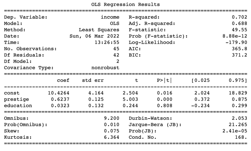

Where does the confidence interval parameter come from? What about the std error, t statistics, and the p-value that is associated with each coefficient? Where do they come from? In this post we are going to take a look on how does this probability metrics came about.

Random variables in linear model

Probabilistic metrics exist with the notion of random variables. In linear regression, the variable of interest \(y\) that we want to predict is assumed to be generated from a normal distribution. In mathematical form, it looks like this:

This form can be rewritten as:

where \(X\) is our observed dataset, \(w_{true}\) is the true parameter that we cannot observe, and \(\epsilon\) is an independent noise.

Why does it looks like this? Why does we have to assume that \(y\) sampled from a normal distribution? The short answer is because we assume linear regression to have this property. In reality, we will never know the value of \(w_{true}\), hence we want to approximate \(w_{true}\) by looking at the observed data \(X\). To do that, we introduce a new variable called \(w_{opt}\), the parameter that we can calculate from observed data. I would assume the reader is familiar with the closed form solution to find the optimal \(w_{opt}\) that approximates \(w_{true}\). The equation is given as:

where the \(Y\) is the label observations in the data. Notice the difference here: \(y\) is a random variable sampled from a normal distribution, whereas \(Y\) is the label observations in the data. We assume that the observed \(Y\) does not equal to \(X w_{true}\), but rather to \(X w_{true}\) plus some corrupted gaussian noise \(\epsilon\). Hence, we further assume that \(Y\) is the observations that we get from sampling the random variable of interest \(y\).

If we look closer to the equation above, we will notice another thing: \(w_{opt}\) is calculated by linearly transforming two components: \(X\) and \(Y\). Since we model \(Y\) as a sample from the random variable \(y\), we can introduce another random variable \(\hat{w}\) that is calculated as:

\(\hat{w}\) represents a distribution of learnt parameter values. \(w_{opt}\), the variable that we use to approximate \(w_{true}\), can be seen as a sample from the distribution of learn parameter values \(\hat{w}\). This is because \(\hat{w}\) is defined as a linear transformation from the random variable \(y\), with \((X^T X)^{-1} X^T\) being the transformer matrix. And since \(Y\) is a sample from \(y\), \(w_{opt}\) is defined by applying the same transformation to the sample \(Y\).

Probability density function for \(\hat{w}\)

Now we want turn \(\hat{w}\) into a probability density function. To get that, we can apply multivariate gaussian linear transformation rule to \(y \sim \mathcal{N}(\mu, \epsilon)\). I will not go into the details of the derivation in this post. For those interested, please see here. Applying the transformation rule yields:

where \(\eta^2\) is the variance of each single random variable \(\epsilon\). It is defined by

where \(\mathbb{I}\) is the identity matrix. In this case, \(\epsilon\) that we introduce in \(y \sim \mathcal{N}(\mu, \epsilon)\) is a multivariate Gaussian noise where it represents noise that is independent at each data point. Hence, the dimension of \(\eta^2\) is \(n\), where \(n\) is the number of data points.

This leaves us with two unknown parameters that we need to define, namely \(w_{true}\) and \(\eta^2\), before we can get the probabilistic metrics out of \(\hat{w}\).

For \(w_{true}\), we use \(w_{opt}\) as it is only sample that we observed in the training data. For \(\eta^2\), we need an observable value for the calculation. Since we already know that \(\hat{w}\) is transformed by the random variable \(y\), we use the variance of \(y\) to represent the noise part for unknown parameters \(\eta^2\). By definition, the variance of \(y\) is the same as the variance of \(\epsilon\) which is the same as the variance of \(\eta^2\). The variance of \(y\) can be calculated by taking the predicted value \(\hat{Y} = X w_{opt}\) versus the observed value \(Y\). Plugging this into a standard deviation formula, we get:

Note that \(\eta^2\) becomes a scalar now. That’s it! We can now proceed to look at each of the probabilistic metrics

Standard deviation

We have defined this above. The standard deviation of our weight distribution is given by \((X^T X)^{-1} \eta^2\). The \((X^T X)^{-1}\) matrix is of p x p dimension and \(\eta^2\) is a scalar, yielding a p x p matrix, where \(p\) is the number of features that we have. The variance of each feature is at the main diagonal of this matrix.

Confidence interval

Since \(\hat{w}\) is a multivariate Gaussian random variable, the confidence interval for each univariate random variable in \(\hat{w}\) is just some standard deviation away from its mean. We use the standard deviation parameter that we have computed above to calculate the confidence interval. For the mean, we use each elements in the \(w_{opt}\) vector.

T-statistic and \(P > t\)

These two metrics measure how likely the mean of the parameter is \(0\). Having a \(0\) mean indicates that the feature does not contribute to predicting the target variable \(Y\). The \(P > t\) is the p-value telling us how far is our mean parameter from \(0\), represented by t-statistics. High p-value tells us that the parameter is unlikely to be meaningful for the prediction, whereas low p-value tells us that the parameter is likely to have high contribution to the prediction.

We calculate the t-statistics of the feature by:

where \(\mu_j\) is the j-th feature mean and \(\eta_j\) is the j-th standard deviation of the j-th feature. To get the p-value of the j-th feature we evaluate the t-statistics under \(\mathcal{N}(0,1)\)

Closing

There were more stuff going on under linear regression that I hadn’t realized before. I hope this post can help you in understanding where does the probabilistic metrics came from.