Have you ever wondered how search engine works? How can they match a query with millions of documents super fast and return them in a personalized way for each users? There are a lot of engineering techniques that power a search engine.

In this post, we are going to look at two components of a search engine. In a simplified view, search engine is composed of two main parts: retrieval and reranking.

Retrieval

In retrieval, we want to return a smaller pool of documents from the huge pools given a query. We essentially want to reduce the number of document candidates that can potentially be of interest according to a given query.

There are many techniques to do retrieval, but the key point is retrieval needs to be fast. In Big-O notation, we want the retrieval to have a time complexity in \(\mathcal{O}(1)\) or at most in \(\mathcal{O}(\log N)\). Higher time complexity yields to slow and unpleasant experience for users.

Retrieval with inverted index

For the sake of simplicity, let’s assume that the query and documents that we have are of string types. To do retrieval fast, we create an inverted index which stores every unique token (vocabulary) that can be found in the document pool and points to document subset containing this token.

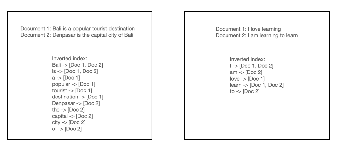
So instead of doing a string match of each query term to the document term, we can directly access the index to return the list of documents of matched query in \(\mathcal{O}(1)\) time complexity.

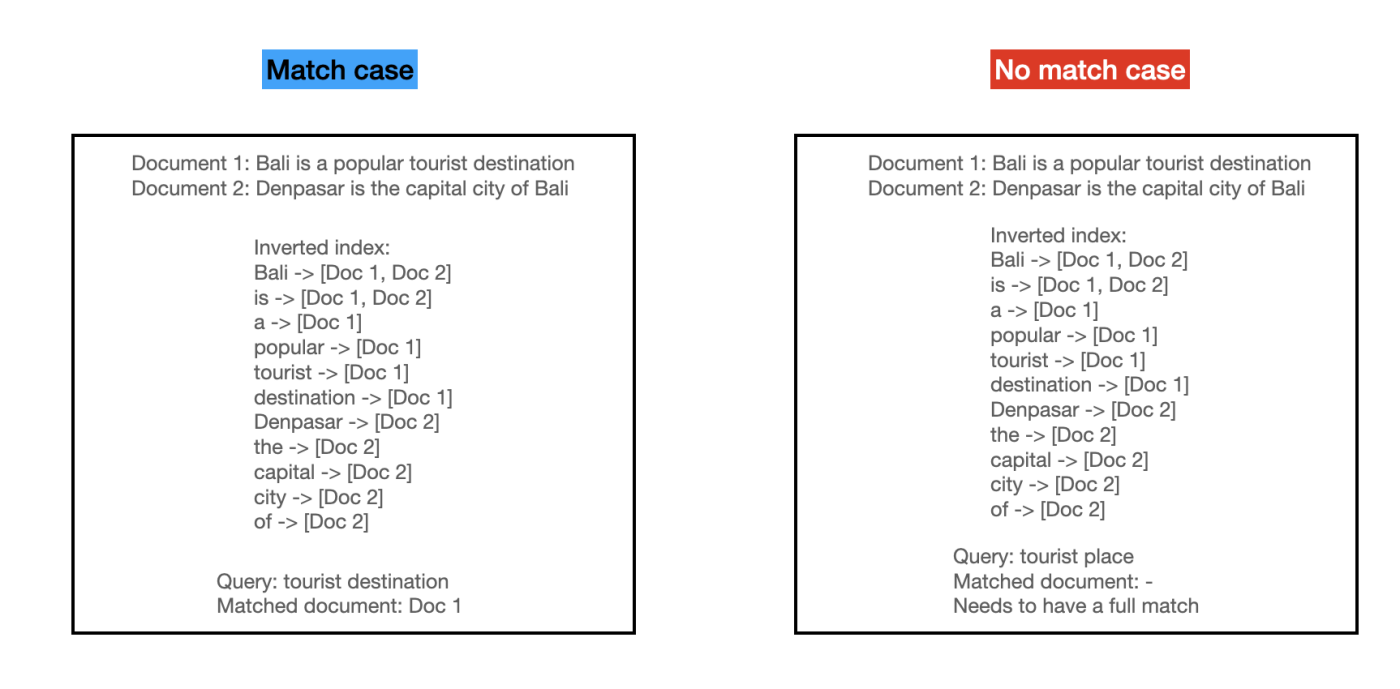
In popular search libraries such as elastic search, we can adjust further on preprocessing (e.g., tokenizing) and on how to define the match. For preprocessing, we can stem words to only include base word, tokenize word using different delimiters, and many more. For match definition, we can determine whether we want full match of all query term, partial match only, or any other heuristics. These heuristics give you some control on which criteria you want the documents to be returned.

Reranking

We need to assign a score to each of the retrieved documents so that we can get the rank from the most relevant items the least relevant items with respect to the query term. There are many ways to assign score to each retrieved documents, from the older approach like tf-idf and bm25 to the more neural network approach. In this post, we’ll take a look at tf-idf.

TF-IDF scoring

As the name suggest, there are two components in tf-idf: term frequency - inverse document frequency.

Given a word \(t\) and document \(d\), term frequency \(f_{t,d}\) is simply the number of times each word \(t\) appeared in document \(d\). The term frequency \(f_{t,d}\) is given as:

Inverse document frequency measures how rare \(t\) is across the corpus \(D\). Given \(N = D\) as the total number of documents in the corpus and \(n_t\) as the number of documents having \(t\), the \(idf(t,D)\) can be calculated as:

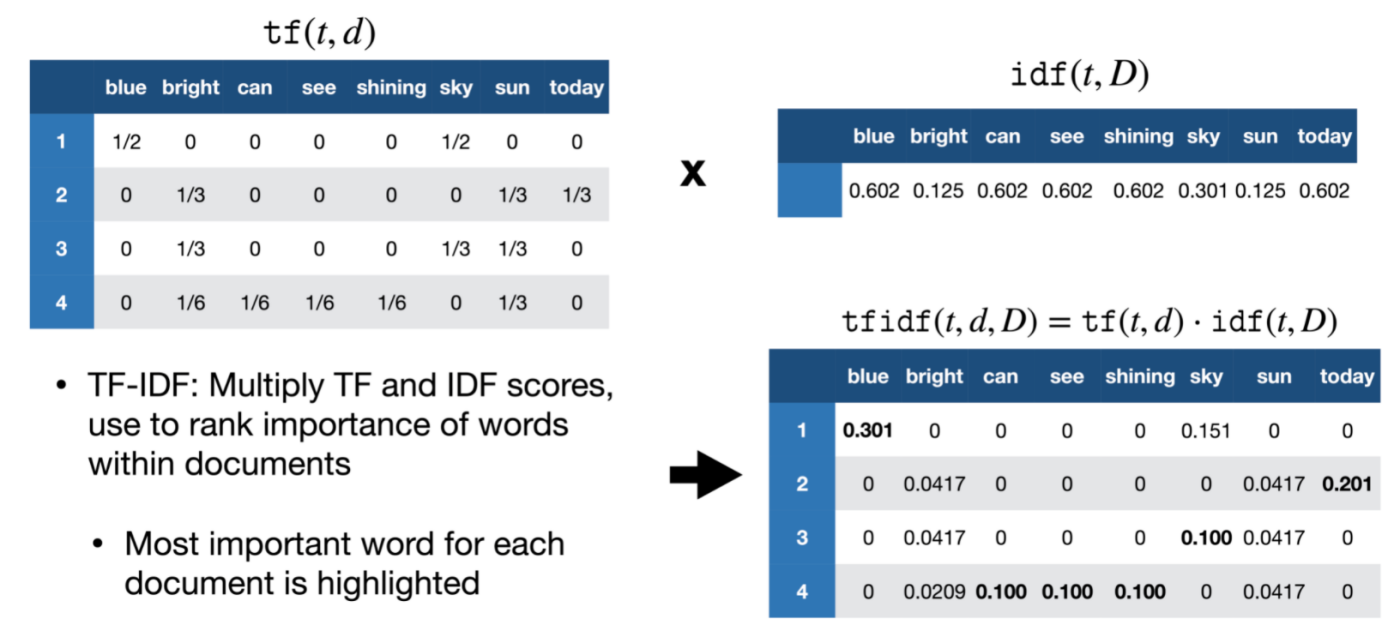
Then we multiply them together to get the tf-idf score:

Calculate tf-idf score for new query

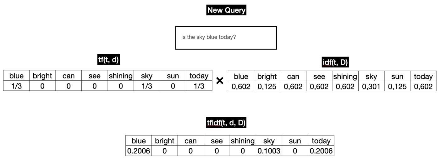
Say that your system is running in production, how does it work when you have new query coming in? For term frequency (tf) we need to calculate it real-time. For idf, we can just use the precomputed idf. See the illustration below:

Once we have the tf-idf vector, we still need to calculate the similarity between the query and the matched product tf-idf vectors. This will result in a complexity of \(\mathcal{O}(m * k)\) where m is the number of matched products and k is the complexity of the similarity metrics (cosine, euclidean, etc). To further speed up this process, we can use approximate nearest neighbor (ANN) which runs in \(\mathcal{O}(\log m * k)\). The details of ANN is out of the scope of this post.

Closing

In the next post we will see other techniques involving retrieval and reranking. Stay tuned and thanks for reading!

Image source for Figure 4,5 and 6.