Decision tree is the crux of many popular algorithms in data science: xgboost, lightgbm, catboost, etc. In this post I aim to explain how decision tree works in both classification and regression setting. This post is meant as a learning notes also for myself.

Classification decision trees

Given series of features \(X\) and a categorical label \(Y\), decision tree works by finding which feature in our instances to split and further divide the instances so that we have a leaf that represent the final prediction. For classification trees, we usually do the split based on a technique called gini impurity (the most popular technique). In practice there are several ways to calculate the split for a leaf. Deciding a split based on gini impurity involves several steps:

• Calculate gini impurity for a leaf
• Calculate total gini impurity for a split
• Decide the split based on feature that has the lowest total gini impurity.
• Repeat step 1-3 until convergence / stopping criteria

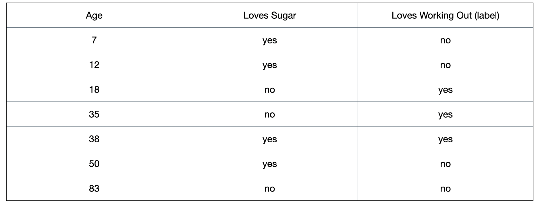
Figure 1: A toy dataset that is used to illustrate the classification section.

Gini impurity for a leaf

Gini impurity for a leaf is calculated as:

where \(p_{c}\) is the class probability and \(C\) is the total number of class. For binary classification, the equation would become:

where \(y_1\) is the yes class probability and \(y_0\) is the no class probability.

For example, if we split the dataset on the “loves sugar” column, we would have:

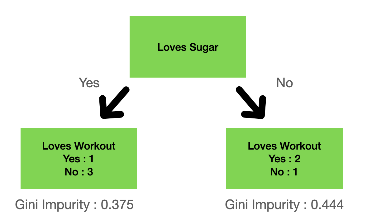
Figure 2: A split example on the “loves sugar” column.

where the gini impurity for the left leaf is given by:

and the right gini impurity:

Total gini impurity for a split

Once we have the gini impurity for each leaf, we need to calculate the gini impurity for a split. Note that these two are different quantities. The gini impurity for a split is the quantity that we use to decide which feature we want to split our instance first. To assess the total gini impurity for a split, we do a weighted average of gini impurities for each leaves:

The idea behind gini impurity is that the more homogeneous sample that we can divide based on a split, then the more pure the split is, hence the lower gini impurity score (0 being the most pure).

Gini impurity for multi categorical variable and numeric continuous variables

For categorical variable with category greater than 2, we calculate gini impurity for every possible split. For example, if we have a categorical variable with value 1,2, and 3, we split:

• based on 1 and not 1 (2 and 3)
• based on 2 and not 2 (1 and 3)
• based on 3 and not 3 (1 and 2)

and then we follow the exact same steps as above. The idea is to binarize the split so that we can calculate the leaf gini impurity and split total gini impurity. The same thing also applies to continuous variable. Coming back to our example, “age” column is a numeric continuous variable. To make a split on that variable, we do something like this:

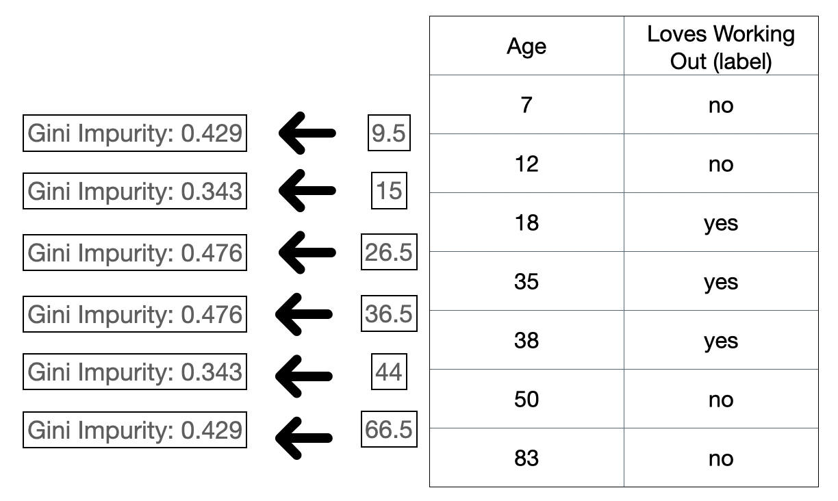
Figure 3: Gini impurity for continuous variables.

Note that we do this on a sorted column because we want the split to be on the sorted instances. The idea is that we decide a split criteria for the continuous variable and we do the exact same steps as the above: treating the split as a binary choice. In the above case, the split criteria is computed based on the mean of every adjacent instances. After we get the mean we then split the instances and calculate the gini impurity like in Figure 2. In practice, there are many ways to decide the split criteria.

Choosing the split

Based on the example above, we have multiple split criterias and their gini impurity scores. We choose the split that has the lowest gini impurity and made it our first split.

Adding branches

We do the same thing as above but now we only consider samples that are included in the node. As we split more, the instances that end up in the leaf will be smaller and smaller.

Deciding when to stop (adding leaves)

We stop when we consider a leaf contains only homogeneous instances. We do not need to split more if all instances on a leaf already belong to one label. We can also stop based on some stopping criteria, for example, by maximum depth. Know when to stop is related to overfitting issue. Splitting perfectly on a training set lead to overfitting whereas splitting fewer lead to underfitting. If by stopping criteria we end up with impure leaf (3 yes label and 1 no label) then we take the majority as the decision.

Do classification decision trees have probabilities?

It is easy to fall into thinking that a classifier always have a probability interpretation. But decision tree is a non-parametric model. It does not have a probabilistic interpretation. One might get a pseudo-probability based on an impure node.

Regression decision trees

For regression trees, the leaf produces a continuous value, which is usually an average \(y\) over the splitted samples. Therefore, to evaluate the split, the sum of squared residuals (SSR) of every splitted samples are usually used. These are the steps:

• Calculate the average predicted value of a leaf
• Calculate sum of squared residuals (average predicted value - sample value) of every samples in both sides of the split
• Decide the split based on a feature that has the lowest sum of squared residuals
• Repeat step 1 -3 until convergence / stopping criteria

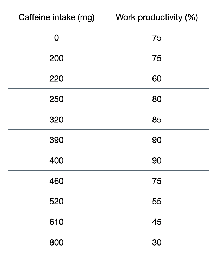
Figure 1: A toy dataset to illustrate this regression section.

Deciding the values to split our feature/column

In regression trees, we do this by sorting the column of our features and then we take the average of the adjacent value. This average value will be our threshold to split our feature into two groups. After the split, we calculate the average predicted value of the leaf.

Sum of squared residuals

After we get the average predicted value of the leaf, we then calculate the sum of squared residuals, which is given by:

where \(y\) is our label and \(f(x_{i})\) is our prediction value. Here the prediction depends on the average predicted value of the leaf/ where the sample ends up after being splitted.

Refer to the two figures below for an example of how to do calculate sum of squared residuals for a split:

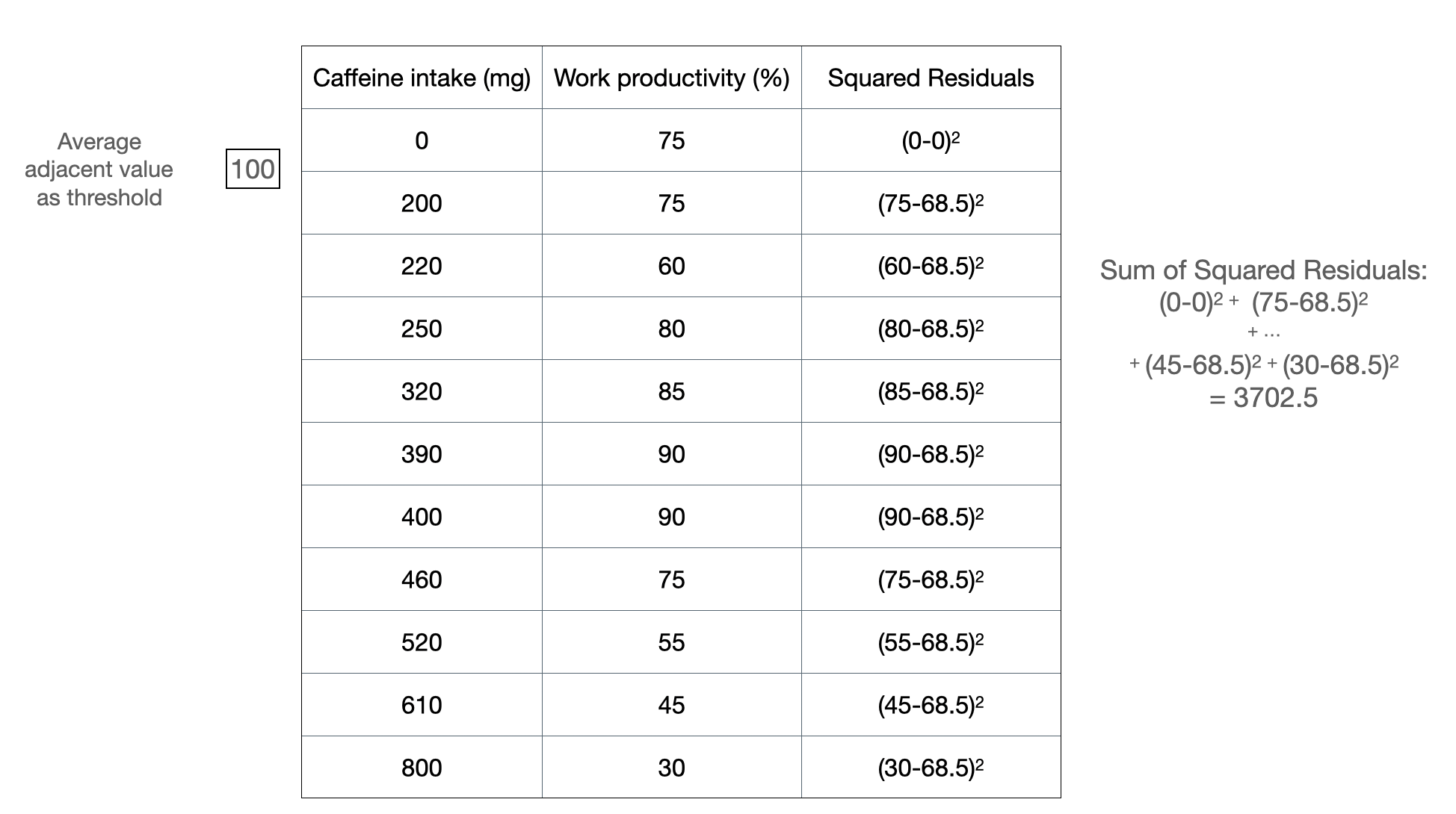
Figure 2a: Example of splitting at a threshold value.

Figure 2a shows how we can calculate a sum of squared residuals for one threshold split, which is at 100 mg. We do this for all possible threshold value for this column:

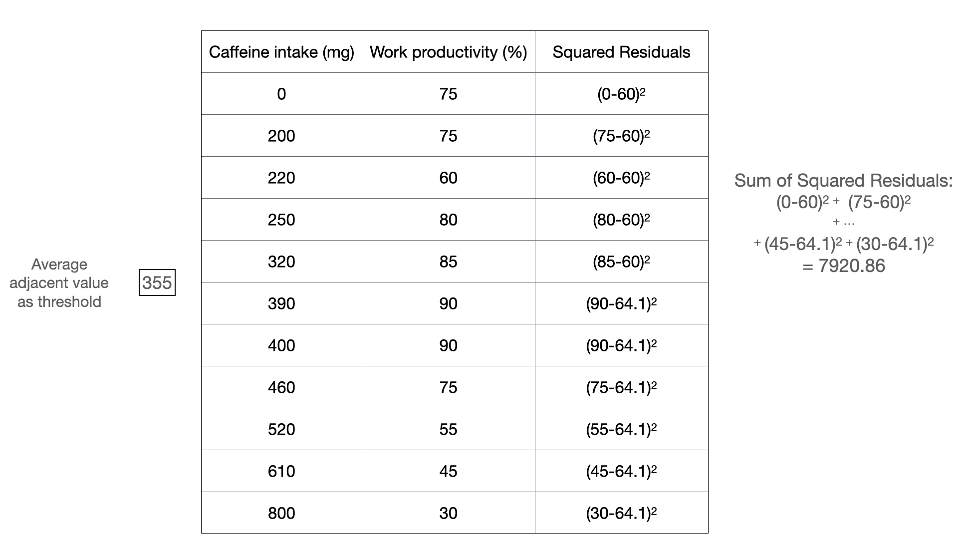
Figure 2b: Another example of splitting at a threshold value.

Choosing the root for both single variable and multiple variables

If we have multiple variables, we do the same as above for every variable possible and we choose the split that has the lowest sum of squared residuals. If we have a binary column, we are just doing one split. Remember that the idea of a split is that we split the instances into two groups and then we move further from there.

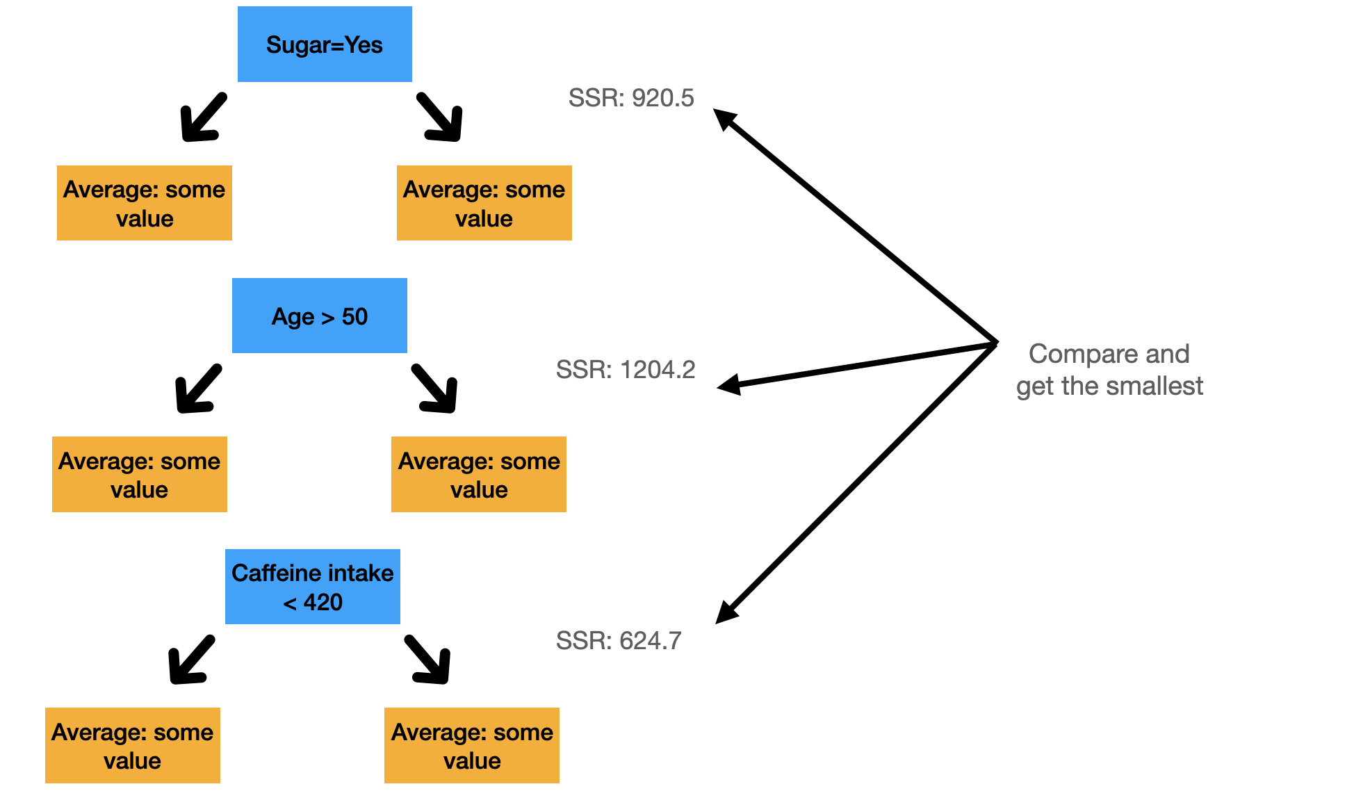
Figure 3: Illustration to get the smallest SSR in multiple variables. The values are all made up.

Adding branches

We do the same thing as in the classification decision tree. Further split only consider samples that are included in the node. As we split more, the instances that end up in the leaf will be smaller and smaller.

Deciding when to stop (adding leaves)

There are multiple ways to do this. The most common one is that we stop when there are less than \(k\) instances in the leaf. \(k\) is usually set at 20. We can also stop based on some stopping criteria, for example, by maximum depth. Know when to stop is related to overfitting issue. Splitting perfectly on a training set lead to overfitting whereas splitting fewer lead to underfitting. With stopping criteria we then take the average \(y\) values of every instances in the leaf and use that as our prediction.

Closing

Decision tree is a non-parametric model that powers several most popular models in data science. In practice, there are many ways to decide which features to split. This post highlights one of the most popular technique for splitting: gini impurity for classification and sum of squared residuals for regression.