AB test is one of the integral parts that a data scientist need to master. One of the goals of doing AB test is to better inform the team to help them make decision. How can we do that? In a hypothetical scenario, let’s say that we have done an AB test and we have gathered two experiment data: one for variant A (baseline) and one for variant B. One of the things that we had to consider is how to analyze the data after the test had run? How do we decide which variant is better? Deciding which variants are better is crucial because ultimately this information is going to influence the team decisions. In this post we are going to see an overview on how we can derive conclusion of an experiment based on the frequentist school of statistic. We will use normal distribution as a distribution to work with as it is one of the most common distribution that we might encounter in a real life AB test.

Before hypothesis testing

Before doing hypothesis testing, the first thing that we need to understand is that we only have samples from our AB test, not the true underlying distribution. Ideally, we want to do the hypothesis testing using the true underlying distribution. In reality, we do not know anything about the true underlying distribution. We do not know their distribution, let alone the parameters of the distribution. All we can do is to make an assumption about: 1) the form of the true distribution and 2) the approximation of the true parameter of the assumed distribution. The former is mostly decided by looking at the problem and data format, whereas the latter is based on the data samples. For example. if we are working with a normal distribution, then we need to know the true mean. We can then make an assumption that the mean can be approximated with our samples. Same thing can also be said for the standard deviation.

Samples

Say that we are making an intervention to our systems and our metric of interest are a continuous value, such as response time of a customer, time it takes for customer to complete an order, etc. We have gathered the experiment data and we assume that the true baseline has mean=0.1 and the true variant b has mean=-0.1.

a = np.random.normal(loc=0.1, size=10000)
b = np.random.normal(loc=-0.1, size=10000)
sns.histplot([a,b],kde=True, bins=50, edgecolor=None)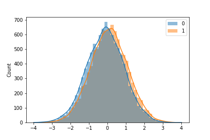

Inferring the parameter: standard error

First we need to infer the parameter of the distribution. In real life we do not know the true parameter, so here we just take the mean and calculate the standard deviation and assume that these values are the true parameter:

a.mean(), a.std(), b.mean(), b.std()
(0.10209145722536886, 1.004581515836704)
(-0.10367983213074679, 1.008924455645851)

With the parameter information at hand, we can plot both distribution with their confidence interval:

a_mu, a_std = a.mean(), a.std()
a_se = a.std() / np.sqrt(len(a)) // standard error
a_ci = (a_mu - 2 * a_se, a_mu + 2 * a_se)

b_mu, b_std = b.mean(), b.std()
b_se = b.std() / np.sqrt(len(b)) // standard error
b_ci = (b_mu - 2 * b_se, b_mu + 2 * b_se)

x = np.linspace(a_mu - 4*a_se, a_mu + 4*a_se, 100)
y = stats.norm.pdf(x, a_mu, a_se)
plt.plot(x, y)
plt.vlines(a_ci[1], ymin=0, ymax=1)
plt.vlines(a_ci[0], ymin=0, ymax=1, label="A 95% CI")

x = np.linspace(b_mu - 4*b_se, b_mu + 4*b_se, 100)
y = stats.norm.pdf(x, b_mu, b_se)
plt.plot(x, y)
plt.vlines(b_ci[1], ymin=0, ymax=1)
plt.vlines(b_ci[0], ymin=0, ymax=1, label="B 95% CI")

plt.legend()
plt.show()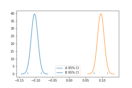

Since we only have one mean, which is our sample mean, we use standard error to create a confidence interval around the sample mean. The confidence interval relies on a theory called central limit theorem. This theorem states that means of experiments are normally distributed. The standard error of the mean serves as our estimate of the distribution of the experiment means. So, if we multiply it by 2 and add and subtract it from the mean of one of our experiments, we will construct a 95% confidence interval for the true mean. Note that we don’t need to restrict ourselves to the 95% confidence interval.

What we can see from Figure 2 is that the 95% CI of the variants don’t overlap. The lower end of the CI for variant b is above the upper end of the CI for baseline. This is evidence that our result is not by chance, and that the true mean for variant b is higher than the true mean for baseline. In other words, we can conclude that there is a significant increase in our metric when switching from baseline to variant b.

Inferring the parameter: bootstrap

There is another way to estimate the interval of the true mean. Ideally when we want to estimate the interval of the true mean, we would like to be able to simulate an experiment with multiple datasets. In other words, we would like to be able to get multiple sample means from different samples to get the mean of means. Using this mean of means, we can then create a confidence interval. This technique is commonly known as bootstrap. I am not going into the bootstrap detail in this post.

Concluding the test using hypothesis testing

To solidify our conclusion regarding confidence interval, we can state a hypothesis test: is the difference in means statistically different from zero (or any other value)? To achieve this, we need to test our the difference between the two distributions against a null hypothesis. The null hypothesis in this case is a zero difference in mean, represented by a zero-centered normal distribution. To calculate the difference between the two distributions, we recall that the sum or difference of 2 independent normal distributions is also a normal distribution. The resulting mean will be the sum or difference between the two distributions, while the variance will always be the sum of the variance.

diff_mu = b.mean() - a.mean()
diff_se = np.sqrt(b.var()/len(b) + a.var()/len(a))
ci = (diff_mu - 1.96*diff_se, diff_mu + 1.96*diff_se)
print(ci)

(0.16824798031433202, 0.22381185401183407)

x = np.linspace(diff_mu - 4*diff_se, diff_mu + 4*diff_se, 100)
y = stats.norm.pdf(x, diff_mu, diff_se)
plt.plot(x, y)
plt.vlines(ci[1], ymin=0, ymax=.05)
plt.vlines(ci[0], ymin=0, ymax=.05, label="95% CI")
plt.legend()
plt.show()

With this at hand, we can say that we are 95% confident that the true difference between the baseline and variant b group falls between -0.22 and -0.17. We can also construct a z statistic by dividing the difference in mean by the standard error of the differences. The z statistic is a measure of how extreme the observed difference is. To further test our hypothesis that the difference between the two means is statistically different, we will assume that the opposite is true, that is, the difference is zero. This is our assumed null hypothesis. Under the null hypothesis, if the difference is indeed zero, we will see the z statistic falls between 2 standard deviations of the mean 95% of the time. If the z statistic falls outside the 2 standard deviations, then we can reject the null hypothesis and conclude that there is a difference between our two distributions.

z = diff_mu / diff_se

x = np.linspace(-4,4,100)
y = stats.norm.pdf(x, 0, 1)
plt.plot(x, y, label="Standard Normal")
plt.vlines(z, ymin=0, ymax=.05, label="Z statistic", color="C1")
plt.legend()
plt.show()

This looks like a highly extreme value. It is below -2 which means there is less than a 5% chance that we would see such an extreme value if there were no difference in the groups. The probability of the z statistic plus the probability of observing more extreme values under the null hypothesis are mostly known as p-values. P-values measure how unlikely it is that we are seeing a measurement if the null hypothesis is true. In our case above, we can see from the graph that our p-value is extremely low (\(2.5*10^{-45}\) to be exact). This again leads us to conclude that switching from baseline to variant b causes a statistically significant improvement in our metric.

print("P-value:", stats.norm.cdf(z))

ttest_ind(a, b)

# the two code above will yield the same value

Closing

To the naked eye, this might shock us as the sample distribution highly overlaps in Figure 1. Personally. I think that p-value is just one component that we can calculate to help make a decision. It should not be the sole reason to decide on a problem. There may be a case where getting an improvement from -0.01 to 0.01 is not necessarily a good thing. So please be careful and know the downside of using p-value.

Thanks for reading my blog post. In the next post, I will talk about frequentist hypothesis testing using a bernoulli distribution. Stay tuned!

Contact me on twitter @rezkaaufar