In the previous post we talked about how does frequentist hypothesis testing work in an AB test using a normal distribution. In this post we are going to look at the hypothesis testing if your variable of interest is binary using a binomial distribution. Let’s get started!

Samples & Parameter Inference

Let’s say that we have completed an AB test and we have sample size \(n=10000\) for both the control and variant group. The control have \(ns_c=5500\) and the variant have \(ns_v=5700\), which represents the number of success we get.

To do a hypothesis test, we need to infer the parameter of the binomial distribution for both the control and variant group. In binomial distribution, the parameter is \(\theta\), which represents the probability of getting a positive outcome in a trial. Based on the data, we can infer that:

\[p_c = \frac{ns_c}{n} = \frac{5500}{10000} = 0.55\] \[p_v = \frac{ns_v}{n} = \frac{5700}{10000} = 0.57\]

Binomial Distribution & Significance Testing

Now we want to determine whether the difference between control and variant group is significant enough so that we can decide which group we want to apply in our system. To do this, we need to find out what is the probability of getting 5700 success (the variant group parameter) assuming that the control distribution with \(p_c=0.55\) is true. Mathematically, it is defined as:

\[a(ns) = \sum_{K=ns}^N {N \choose K} P_{0}^{K} (1 - P_{0}^{K})^{N-K}\]

where in this case \(ns\) is the variant group successes \(ns_v\) and \(P_0\) is the control group binomial distribution parameter \(p_c\).

In plain words, the formula tells us what is the probability of observing the event plus the probability of observing other events that are equally rare and more extreme. In this case, the event is the variant group successes \(ns_v\). Also note that I am using a one-sided test because in an AB test we only care about getting an improvement. We don’t care if the variant group successes is significantly worse than control group success, even though by statistical definition it still counts as significant.

from scipy import stats
stats.binom_test(5700, n=10000, p=0.55, alternative='greater')
2.9637380107656557e-05

Using python code above, we can see that we get a low p-value, which tells us that it is unlikely to get 5700 successes assuming that the control distribution is true. Hence we can conclude that the variant group yields better conversion.

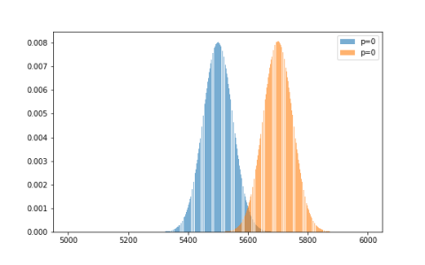
Figure 1: Gaussian approximation of binomial distribution of both the control and variant group.

Figure 1 shows the gaussian approximation of both the control and variant binomial distributions. By theory, we know that we can approximate binomial distribution with a normal distribution. In math notation, the parameter of the normal distribution can be calculated as:

\[\mu = np\] \[\sigma = np(1-p)\]

where \(n\) is the number of trials and \(p\) is the probability of success in a trial.

We can use \(\sigma\) to calculate the confidence interval around the binomial parameter:

p = 0.55
n = 10000
SE = np.sqrt(p*(1-p)/n)
print(f'95% confidence interval of our binomial distribution is between {np.round(p - 2*SE, 2)} and {np.round(p + 2*SE, 2)}')
95% confidence interval of our binomial distribution is between 0.54 and 0.56

The confidence interval reinforces our initial findings that getting \(0.57\) is unlikely assuming that \(p_c=0.55\) is true.

Closing

Thanks for reading my blog post! Hit me on twitter @rezkaaufar.