Notes on doing AB test properly

February 7, 2026 · 8 min read · statisticsexperimentation

I have known AB Testing and used it for a while in my work but sometimes I find myself remembering the equation too much and unsure about how things worked under the hood. In this post I try to go over the concept and visualize it to make it easier to remember.

MDE, power, alpha, and sample size

We start off by looking at the relationship between minimum detectable effect (MDE), power (1-beta), alpha, and sample size. In an AB test, we set MDE, power, and alpha to calculate the minimum sample size required to run the AB test.

Here is an image showing the relationship between the 4 variables:

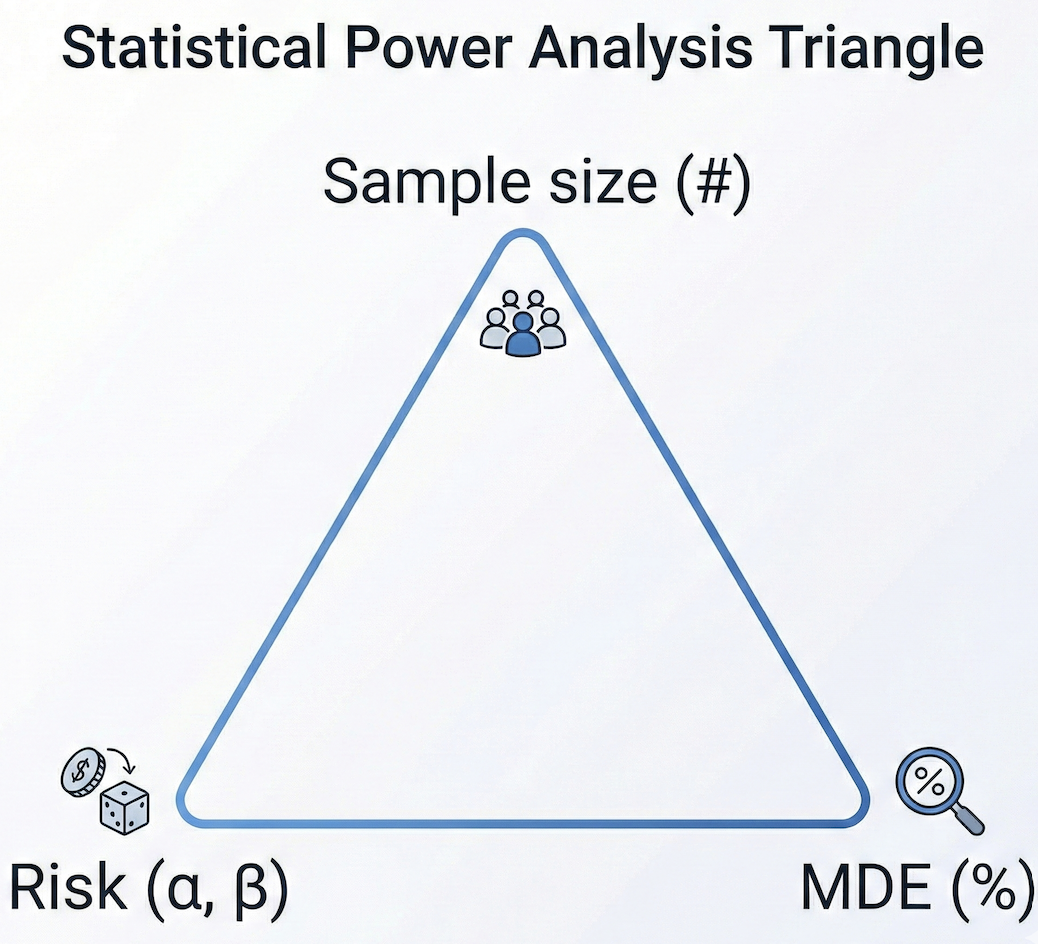
Figure 1: Statistical power analysis triangle. A change in one variable requires fixing the other two

Before we go to the sample size calculation, we start off by varying sample size and see how it affects the distributions of the control and treatment groups.

We begin with two distributions of a conversion metrics, one for the control group and one for the treatment group. Here is the detail of our distributions:

p_base = 0.1
p_treat = 0.12
se0 = np.sqrt(p_base * (1 - p_base) / n)
se1 = np.sqrt(p_treat * (1 - p_treat) / n)

Here we assume that our control group conversion is 10% and our target treatment group conversion is 12%. We can plot both our distribution above with varying sample size n:

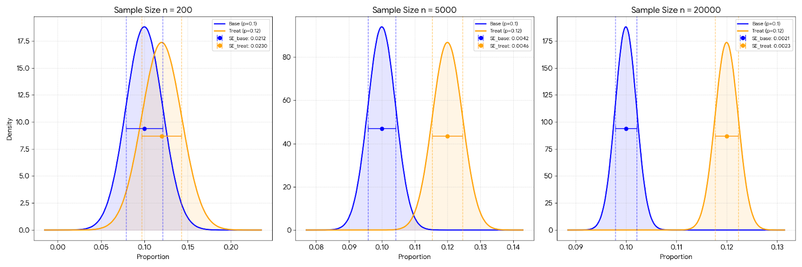
Figure 2: Control versus treatment distribution

We can see that as the sample size increases, the gap between the two distributions also increases. This is because the standard error decreases as the sample size increases. And this will affect our AB testing later.

Now that we have the control and treatment distribution, we can do a hypothesis testing by constructing a third distribution, which is the distribution of difference in the means. I will not go over the theory too deep here, but this approach is based on the Central Limit Theorem, where the distribution of the difference between two means will approach a normal distribution as the sample size increases.

For the hypothesis testing, we calculate three components: the standard error of the difference (se_diff), the null hypothesis (mu0), and the alternative hypothesis (mu1).

# Standard Errors
se0 = np.sqrt(p_base * (1 - p_base) / n)
se1 = np.sqrt(p_treat * (1 - p_treat) / n)
se_diff = np.sqrt(se0**2 + se1**2)

mu0 = 0
mu1 = mde

We set mu0 to 0 because this is our null hypothesis. We assume that there is no mean difference in both control and treatment, whereas mu1 is our MDE, which is the effect that we want to see. Technically, mu1 is calculated like this:

mean_diff = p_treat - p_base
mu1 = mean_diff - mu0

which basically is equal to our MDE. In this phase where we haven’t done any AB testing, we assume that the treatment group is better than the control group by MDE.

Now we can plot the distribution of this mean difference by varying the sample size and observe how it affects our power and how does the shape of the distribution change as we adjust the sample size.

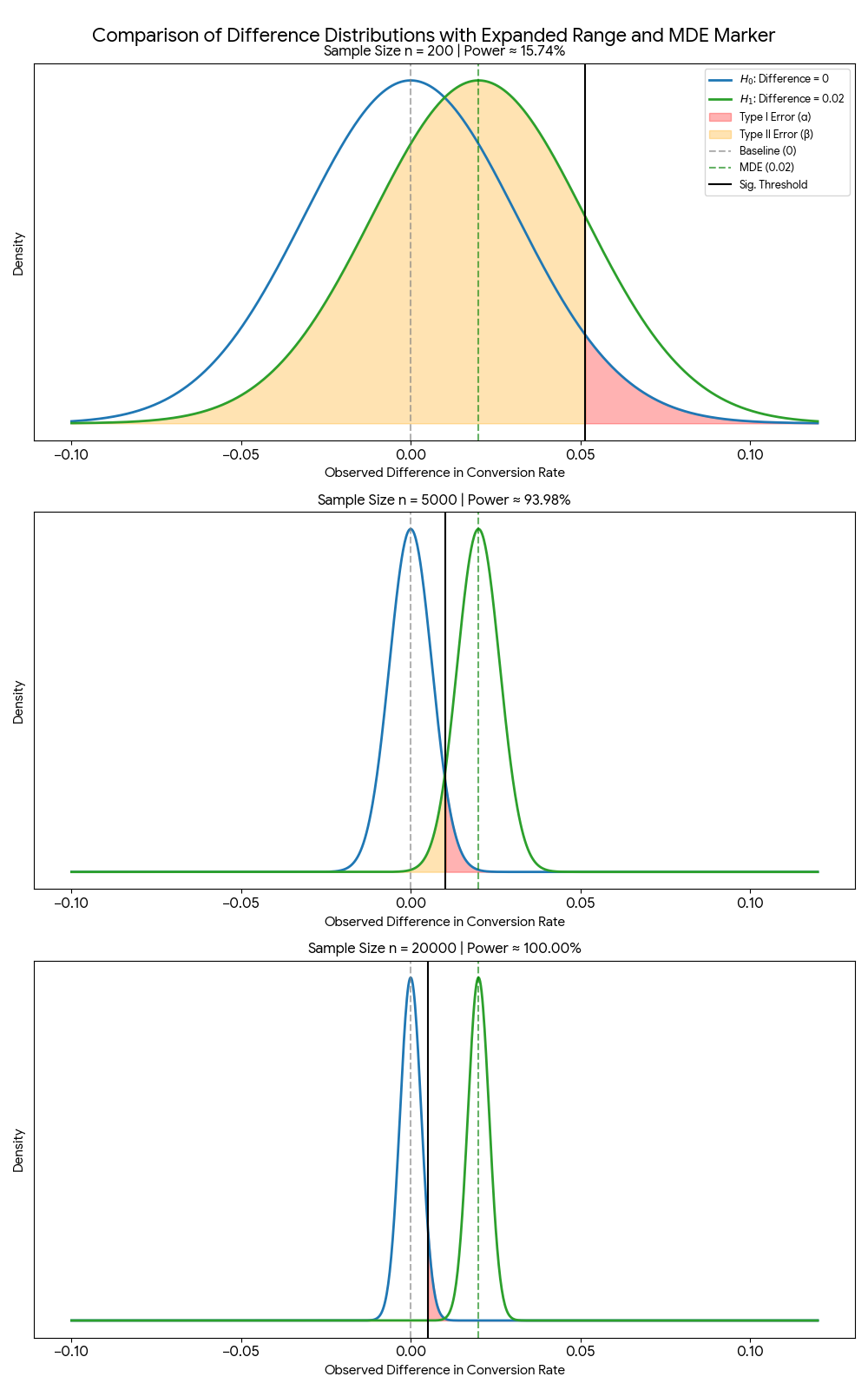Figure 3: Comparison of mean difference distributions with varying samples

The solid black line (threshold) represents the critical value, which is the value that we use to determine if our result is statistically significant. This black line is calculated based on the z-score of the alpha value and the standard error of the difference in means.

# Significance Threshold (Critical Value)
z_alpha = norm.ppf(1 - alpha)
x_crit = mu0 + z_alpha * se_diff

We can see at $n=200$ the threshold is actually to the right of the green dashed line (the MDE). This shows that with such a small sample, even if we hit our exact target of $0.02$, it wouldn’t be “statistically significant.” We would need a massive, lucky fluke to actually reject the null. As $n$ hits $20,000$, the black threshold line moves significantly to the left of our $0.02$ target, meaning almost any result near our MDE will be correctly identified as a winner.

Notice how the power changes as we have increased sample as well. Power is the entire rest of the green curve to the right of the significant line. It represents all the times the treatment actually worked and we correctly identified it as a winner. If we have power of 80%, this means that if the 2% lift is real, we will correctly identify it 4 out of 5 times.

Now we can see that there is indeed a relationship between the MDE, alpha, beta and the minimum sample size required. For a test to be valid in detecting our MDE, we need to have a sample size that is large enough to reject the null hypothesis.

Deciding sample sizes

As mentioned above, in an AB test what we want is to determine the minimum sample size to be able to conclude an experiment given the experiment config. Hence, what we usually do is that we set alpha, beta (power), and our MDE to calculate how many samples do we need to run the AB test.

Here is how the image looks if we do one-tail test with alpha=5%, beta=20%, and MDE of 0.02

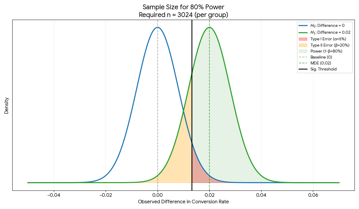Figure 4: Distribution of meandifference when by setting alpha=5%, beta=20%, and MDE of 0.02

Here we observe the following:

At $n=3,024$, the significant threshold is positioned perfectly so that 5% of the Blue Curve is to its right (our $\alpha$ or False Positive risk) and 20% of the Green Curve is to its left (our $\beta$ or False Negative risk)

We can also observe that he curves are just “skinny” enough that the Green Shaded Area (Power) covers exactly 80% of the Treatment distribution. This means if the 2% lift is real, we will correctly identify it 4 out of 5 times.

Concluding the experiment

Once we have our AB test results, we can conclude the experiment by checking if the result is statistically significant.

With the observed $\hat{p}_1$ from our treatment group $\hat{p}_0$ from our control group, and $SE_{observed}$ as the standard error of the difference in means, we calculate z-score

If $Z$ > $Z_{\alpha}$ (1.96 in $N(0,1)$), then we can reject the null hypothesis and conclude that the treatment is statistically significant.

Another way to look at it is to look at our observed $\hat{p}_1$ and if it is above the black threshold ($x_{crit} = 0 + 1.96 \cdot SE_{diff}$) ($\approx 0.013$), then we can reject the null hypothesis and conclude that the treatment is statistically significant.

What to do if your test is statsig but effect size is below your MDE?

In this case, I believe we can reject the null hypothesis. If our result lands slightly to the left of the “True Effect” ($0.02$), as long as it stays to the right of the black threshold ($\approx 0.013$), we can still detect it as statistical significant. It is still good to proceed with the treatment if we observe an increase in our metrics.

If the effect size is positive but it is below the significance threshold (not statistically significant), then this warrants a further decision and investigation. It could be that the true effect size is indeed smaller than the MDE and requires more sample size to detect it. We can consider to continue the experiment with higher sample size if the cost of running the experiment is low and the potential benefit is high. Otherwise, we can consider to stop the experiment and try again with a different approach.

The other case where we should not proceed with the treatment is when we do not reach statistical significance or if the effect size is negative. Negative effect means that the outcome of the treatment is worse than the control.

What happens if we have unequal split between control and treatment?

Lets say we have 90% control and 10% treatment.

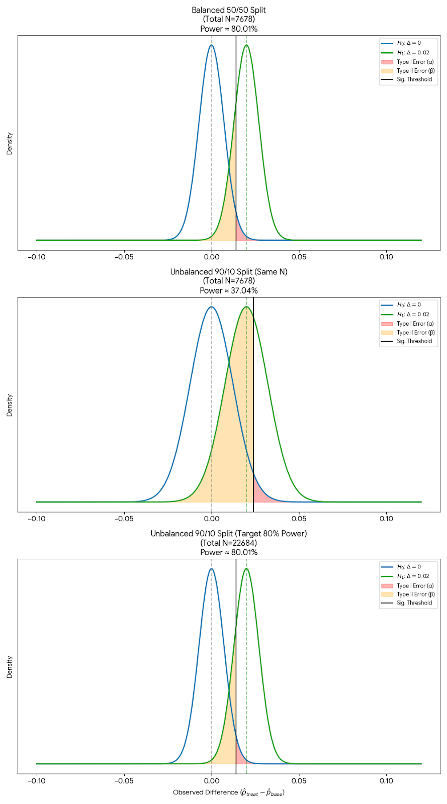Figure 5: Distribution of difference when by setting alpha=5%, beta=20%, and MDE of 0.02 and unequal split between control and treatment

In this case, the standard error of the distribution of the mean difference increases, which means that we need a larger sample size to achieve the same level of statistical significance. So an unequal split in an AB test requires higher samples.

From the formula above, a tiny sample in either group will blow up the total error.

Same case can also be said if we have 10% control and 90% treatment. Even though here we are aggresively rolling out to new users and impacting the main metrics already, the changes cannot be fully trusted until we have enough sample to reach statistical significance.